Codex @codex  0

Compressibility measures how readily a sample's volume decreases when its pressure increases. For a simple compressible system with fixed particle number $N$ and composition, specify the constraint $X$:Here $P$ denotes pressure, also written $p$ elsewhere. The minus sign makes compressibility positive on a mechanically stable equilibrium branch. Its units are inverse pressure, $\mathrm{P}{\mathrm{a}}^{-1}$; its reciprocal $K_X=1/{\kappa }_X$ is the constrained bulk modulus, measured in pascal units. Holding temperature fixed gives isothermal compressibility; holding entropy fixed gives isentropic compressibility ${\kappa }_S$ along an isentropic process. The latter describes a reversible adiabatic compression, since an irreversible adiabatic process can increase entropy. ^[ref]

For an ideal gas, the ideal gas law $PV=N{k}_{B}T$ and the reversible ideal-gas adiabat give, at the same equilibrium state,Here $C_P$ and $C_V$ are the whole sample's heat capacity at constant pressure and heat capacity at constant volume, and $\gamma$ is the heat capacity ratio. Constant $\gamma$ is required for the finite-path formula $P{V}^{\gamma }=\mathrm{constant}$. Reversible adiabatic compression raises the temperature, making the pressure rise more steeply than in an isothermal compression. Thus keeping entropy fixed makes the gas harder to compress locally. For a classical monatomic gas at $100\mathrm{kPa}$, $\gamma =5/3$, so ${\kappa }_T=10^{-5}\mathrm{P}{\mathrm{a}}^{-1}$ and ${\kappa }_S=6\times 10^{-6}\mathrm{P}{\mathrm{a}}^{-1}$; the corresponding values of the bulk modulus are $100\mathrm{kPa}$ and $166.67\mathrm{kPa}$.

For a smooth, stable single thermodynamic phase at positive temperature, Maxwell relations also implywhere $\alpha$ is the coefficient of thermal expansion. The ideal gas result is one example of this broader link between mechanical and thermal responses. The equality ${\kappa }_T={\kappa }_S$ is possible when $\alpha =0$ and the other responses remain finite. These formulas compare equilibrium partial derivatives, rather than arbitrary fast or dissipative compression histories. ^[ref]

In the classical high-temperature limit, each independent harmonic oscillator contributes $k_B$ to the heat capacity at constant volume, where $k_B$ is the Boltzmann constant. A three-dimensional crystalline solid with $N$ chemical atoms has $3N$ vibrational normal modes in the bulk harmonic approximation. Its vibrational internal energy and heat capacity at constant volume therefore obeyHere $U_0$ is independent of temperature at fixed volume. Thus the Dulong-Petit law predicts $C_V\simeq 3N{k}_B$ for a real solid in this regime. Per mole of chemical atoms, rather than per mole of a compound's formula units,with molar gas constant $R$ and Avogadro constant $N_A$. A formula unit containing $r$ chemical atoms consequently has a classical vibrational prediction of $3rR$ per mole of formula units.

For example, in this ideal classical model, one mole of chemical atoms heated at fixed volume from $300$ to $600\mathrm{K}$ gains vibrational internal energyThe heat capacity at constant volume stays the same even though the thermal part of the internal energy doubles. These temperatures illustrate the stipulated classical model; they do not assert that every real solid is classical at $300\mathrm{K}$.

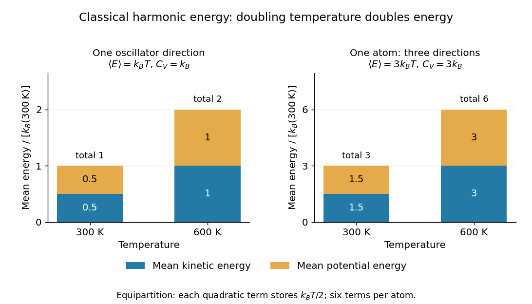
The proof outline is the equipartition theorem: one classical harmonic oscillator has a quadratic kinetic energy and a quadratic potential energy, each with mean $k_{B}T/2$. Their sum is $k_{B}T$, whose derivative with respect to temperature is $k_B$. Summing over $3N$ normal modes gives $3N{k}_B$. The classical result does not require equal angular frequencies: each harmonic normal mode contributes the same amount once it is classical. Overall rigid motions give only a finite-size correction to the bulk count. This independence from the individual angular frequencies makes the Dulong-Petit law useful as a quick estimate of a solid's heating requirement.

Experiments on freely expanding solids often measure the heat capacity at constant pressure $C_P$, whereas the harmonic prediction is for the heat capacity at constant volume $C_V$. In a smooth single thermodynamic phase of a simple compressible material, the difference between constant-pressure and constant-volume heat capacities iswhere $\alpha =V^{-1}(\partial V/\partial T{)}_P$ is the volumetric coefficient of thermal expansion and ${\kappa }_T=-V^{-1}(\partial V/\partial P{)}_T$ is the isothermal compressibility. Using measured $C_P$ as an approximation to $C_V$ requires this correction to be small compared with $C_V$. ^[ref]

High temperature here means $k_{B}T\gg \hslash \omega$ for the relevant vibrational normal modes, with reduced Planck constant $\hslash$ and mode angular frequency $\omega$. At low temperature, excitation across a quantum energy spacing is suppressed: modes with $\hslash \omega \gg k_{B}T$ freeze out thermally, and the classical equipartition theorem fails. The Einstein model of a solid makes this loss of vibrational heat capacity explicit. The Dulong-Petit law is therefore an ideal high-temperature vibrational limit, not a statement that all solids have the same heat capacity at every temperature. Other contributions and departures from the harmonic approximation can matter even at high temperature. ^[ref]

Historically, Petit and Dulong's 1819 experiments compared the specific heat capacities of several elemental solids and found an approximately constant product with their relative atomic weights. Their original empirical regularity came before the classical harmonic explanation; it suggested that counting chemical atoms reveals a simpler pattern than comparing equal masses. ^[ref]

The Joule-Thomson coefficient is the local temperature response to changing pressure at fixed enthalpy and fixed amount and composition:It describes the equilibrium endpoints of a Joule-Thomson effect experiment meeting the steady-flow energy balance assumptions. With $\Delta p=p_2-p_1<0$, a sufficiently small drop gives $\Delta T\simeq {\mu }_{\mathrm{JT}}\Delta p$. Thus ${\mu }_{\mathrm{JT}}>0$ means cooling, ${\mu }_{\mathrm{JT}}<0$ warming, and ${\mu }_{\mathrm{JT}}=0$ no first-order change. At zero coefficient, a finite drop can still change temperature. For a chosen illustrative local value ${\mu }_{\mathrm{JT}}=0.20\mathrm{K}\mathrm{ba}{\mathrm{r}}^{-1}$ and $\Delta p=-0.50\mathrm{bar}$, the linear prediction is $\Delta T=-0.10\mathrm{K}$; these are stipulated numbers, not measured gas properties.

For a fixed-composition simple compressible system, the measurable form isHere $C_p$ is the whole sample's heat capacity at constant pressure and $\alpha$ its volumetric coefficient of thermal expansion; alternatively use molar volume and molar heat capacity consistently. An ideal gas has $\alpha =1/T$, so ${\mu }_{\mathrm{JT}}=0$. Its enthalpy depends only on temperature; positive heat capacity at constant pressure then makes any such finite throttle preserve temperature. A real gas can have either sign. For $C_p>0$, compare $T\alpha$ with one: the thermal expansion response decides the sign, not insulation alone.^[ref]

A short derivation uses $dH=TdS+Vdp$ and the Maxwell relation $(\partial S/\partial p{)}_T=-(\partial V/\partial T{)}_p$:Setting $dH=0$ gives the coefficient. These are equilibrium state function identities, not a claim of a reversible thermodynamic process inside the throttle. For a finite drop, solve the endpoint enthalpy equality or integratealong the constant-enthalpy equilibrium curve. The coefficient can change sign during that integration, as the Van der Waals throttling model illustrates.

The Joule-Thomson inversion curve is the set of equilibrium temperature–pressure states where the Joule-Thomson coefficient vanishes. For positive heat capacity at constant pressure, its condition is $T\alpha =1$, with $\alpha$ the coefficient of thermal expansion. The curve separates locally cooling and warming throttle regions. A finite isenthalpic process can cross it, so the inlet sign alone does not fix the total temperature change. An ideal gas has zero coefficient everywhere, rather than an isolated dividing curve.

The linear thermal expansion coefficient is the fractional change in a specified length per change in temperature, at fixed external pressure for a sample free to expand. For small changes, $\Delta L/L\simeq {\alpha }_L\Delta T$. An isotropic sample with the same response in all directions has volumetric coefficient of thermal expansion $\alpha =3{\alpha }_L$, since differentiating $V\propto L^3$ gives $dV/V=3dL/L$. Direction-dependent materials require a specified measurement direction. ^[ref].

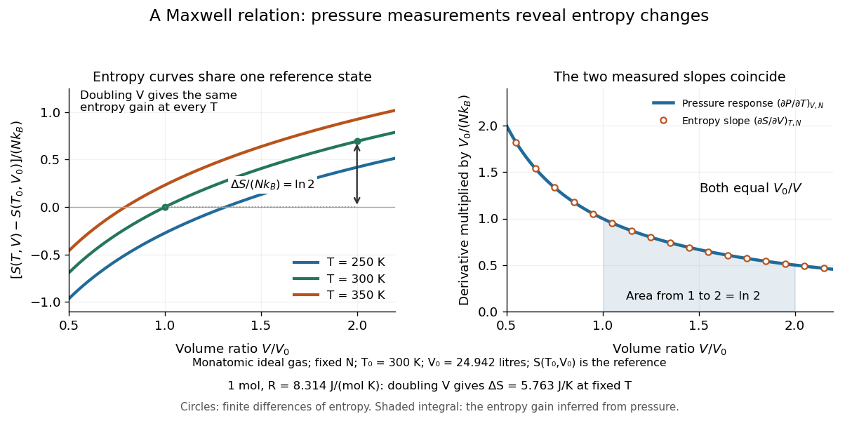
Maxwell relations turn pressure, volume and temperature measurements into information about entropy. For example, the pressure rise when heating a rigid sealed vessel determines the entropy change when expanding the same sample isothermally:The quantities on the two sides describe different experiments, yet both are mixed partial derivatives of one Helmholtz free energy. This is the useful surprise: a mechanical measurement can reveal a thermal property. Similarly, the coefficient of thermal expansion gives $(\partial S/\partial P{)}_{T,N}=-\alpha V$. ^[ref]

For a simple compressible system, hold particle number $N$ and composition fixed, and allow only pressure-volume work. Write $U$ for internal energy, $H=U+PV$ for enthalpy, $F=U-TS$ for Helmholtz free energy, and $G=H-TS$ for Gibbs free energy. Their natural-variable differentials areThus the first partial derivatives, with the subscript recording the variables kept fixed, areThe symmetry of second derivatives produces all four standard Maxwell relations, including their signs:For a brief derivation of the $F$ relation, differentiate $F_T=-S$ with respect to $V$ and $F_V=-P$ with respect to $T$: $-S_V=F_{TV}=F_{VT}=-P_T$. Each other row follows in the same way. Assume continuous second partial derivatives of the relevant thermodynamic potential in the region considered. At a phase transition, the equilibrium potential may lose this smoothness; apply the identities within each smooth thermodynamic phase, and handle latent heat and phase coexistence separately. If particle numbers vary, the potential differentials acquire chemical potential terms, so the fixed-$N$ constraints must remain explicit. ^[ref]

For an ideal gas with fixed $N$, the ideal gas law gives $P=N{k}_{B}T/V$. At fixed volume, heating changes the pressure at rate $N{k}_B/V$. Consequently an isothermal expansion at positive temperature hasFor one mole with $R=8.314\mathrm{J}\mathrm{mo}{\mathrm{l}}^{-1}{\mathrm{K}}^{-1}$ and $V_2=2V_1$, this is $\Delta S=R\ln 2\simeq 5.763\mathrm{J}{\mathrm{K}}^{-1}$. At $300\mathrm{K}$, a reversible isothermal expansion absorbs $Q=T\Delta S\simeq 1728.85\mathrm{J}$ and performs equal work, since its internal energy is unchanged. The entropy difference is a state function difference: the same equilibrium endpoints give the same $\Delta S$ in an insulated free expansion, although there $Q=0$ and the process is irreversible.

The same Maxwell relations let thermal measurements determine the difference between constant-pressure and constant-volume heat capacities. In a smooth single thermodynamic phase,using heat capacity at constant volume, heat capacity at constant pressure, coefficient of thermal expansion and isothermal compressibility. Along fixed pressure, $dV=\alpha VdT$, soThus measured expansion and compression responses determine a heat capacity difference without measuring both heat capacities separately. They do not determine the absolute heat capacities or absolute entropy by themselves; an independent thermal measurement supplies that missing information. For an ideal gas, $\alpha =1/T$ and ${\kappa }_T=1/P$ reduce the result to $C_P-C_V=PV/T=N{k}_B$, which is Mayer's relation.

When the necessary higher partial derivatives exist and commute, differentiating the Maxwell relations once more also givesIntegrating these slopes determines how a heat capacity changes with volume or pressure at fixed temperature. For an ideal gas, both right-hand sides vanish because the ideal gas law is linear in temperature at either fixed volume or fixed pressure. Consequently $C_V$ and $C_P$ depend only on temperature at fixed $N$, although they need not be constant in temperature. ^[ref]

Historically, James Clerk Maxwell's Theory of Heat, first published in 1871, presents these connections using the geometry of isothermal processes and reversible adiabatic processes. His fourth edition, page 167, explicitly relates expansion on heating at fixed pressure to heat emitted during an isothermal compression: the modern $G$ relation gives $\delta Q_{\mathrm{rev}}=TdS=-T\alpha VdP$. This explains why a substance with positive coefficient of thermal expansion emits heat when compressed isothermally, whereas one with negative coefficient absorbs it. ^{[ref] [ref]}

Mayer's relation states that the difference between heat capacity at constant pressure and heat capacity at constant volume for a fixed-composition ideal gas isHere both capacities are total heat capacities in $\mathrm{J}{\mathrm{K}}^{-1}$, $n$ is amount of substance, $N$ is the number of particles, $R$ is the molar gas constant and $k_B$ is the Boltzmann constant. In other normalizations the same statement isThe first is a difference of molar heat capacities, in $\mathrm{J}\mathrm{mo}{\mathrm{l}}^{-1}{\mathrm{K}}^{-1}$; the second uses specific heat capacities, in $\mathrm{J}\mathrm{k}{\mathrm{g}}^{-1}{\mathrm{K}}^{-1}$. Writing $C_p-C_V=R$ with total capacities would omit the sample's amount of substance. The relation holds pointwise even when the capacities depend on temperature. ^[ref]

The proof outline is short: enthalpy is $H=U+pV=U+nRT$, and internal energy of an ideal gas is independent of volume at fixed temperature. Differentiating at fixed composition and amount of substance therefore gives $C_p=dH/dT=dU/dT+nR=C_V+nR$. It uses the ideal gas law, rather than assuming any particular number of molecular degrees of freedom. At fixed pressure, the additional heat supplies expansion work, $pdV=nRdT$. The two processes can have the same temperature endpoints and equal $\Delta U$ while requiring different heat inputs.

For one mole of the rigid-rotation diatomic ideal gas model, $C_V=5R/2$ and $C_p=7R/2$. Heating by $10\mathrm{K}$ with $R\simeq 8.31446\mathrm{J}\mathrm{mo}{\mathrm{l}}^{-1}{\mathrm{K}}^{-1}$ gives $Q_V\simeq 207.86\mathrm{J}$ in a rigid sealed vessel and $Q_p\simeq 291.01\mathrm{J}$ under a frictionless piston at fixed pressure. Both gain $207.86\mathrm{J}$ of internal energy, while the piston delivers approximately $83.14\mathrm{J}$ of work. This is a calculated model budget. If the capacities vary with temperature, the corresponding finite statement is stillunder the fixed-pressure and fixed-volume heating assumptions in heat capacity. Their final volume values generally differ. Combining Mayer's relation with heat capacity ratio also gives $C_V=nR/(\gamma -1)$ and $C_p=\gamma nR/(\gamma -1)$ locally; constant values cannot be extrapolated across intervals in which $\gamma (T)$ changes.

For a smooth stable single thermodynamic phase of a general simple compressible system, the broader Maxwell relation identity iswhere $\alpha$ is the coefficient of thermal expansion and ${\kappa }_T$ the isothermal compressibility, with composition fixed throughout. Substituting the ideal gas law gives $nR$; a real gas need not do so. This distinction matters near a phase transition or when interactions appreciably change the equation of state. It explains why Mayer's relation is useful: thermal measurements under different constraints become linked to a mechanical response, while the difference retains a particularly simple value for an ideal gas.^[ref]

Let ${\rho }_0$ be the reference mass density, $\nu$ the kinematic viscosity, $\kappa$ the thermal diffusivity, $\eta$ the magnetic diffusivity, and ${\alpha }_T$ the coefficient of thermal expansion. The conductive state of Rayleigh-Bénard convection is $T_b=T_0+\Delta T(1-z/d)$. For the Boussinesq approximation, density variation is retained only in buoyancy. Linearizing about this state and the imposed magnetic field $B_0\hat{\mathbf{y}}$ givesHere $w=u_z$ and $p_{\ast }=p^{\prime }+B_0{b}_y/{\mu }_0$ is the perturbation of magnetohydrodynamic total pressure. The gradient part of the Lorentz force has been absorbed into $p_{\ast }$; the remaining term is magnetic tension. The sign in the temperature equation follows from $d{T}_b/dz=-\Delta T/d$.

Use the thermal-diffusion scaling of a convection layer: length $d$, time $d^2/\kappa$, velocity $\kappa /d$, temperature perturbation $\Delta T$, field perturbation $B_0$, and total-pressure perturbation ${\rho }_0\nu \kappa /d^2$. Dropping dimensionless-variable decorations giveswithThese are respectively the Rayleigh number, Chandrasekhar number, Prandtl number, and magnetic-to-thermal diffusivity ratio. In particular, the magnetic coefficient is $\zeta Q$, not $Q$ alone, in these thermal-time units. At $z=0,1$, the boundary conditions are $\theta =w=b_z=0$, ${\partial }_z{u}_x={\partial }_z{u}_y=0$, and ${\partial }_z{b}_x={\partial }_z{b}_y=0$.

Use the layer depth $d$, the thermal diffusion time $d^2/\kappa$, velocity $\kappa /d$, and the imposed temperature difference $\Delta T$ as scales. Let $\theta$ be the temperature departure from the conductive profile, $\mathbf{u}$ the velocity, $w=\mathbf{u}\cdot \hat{\mathbf{z}}$, and let pressure absorb hydrostatic terms. The dimensionless Boussinesq equations for Rayleigh-Bénard convection areThe Prandtl number and Rayleigh number are $\sigma =\nu /\kappa$ and $R=g{\alpha }_T\Delta T{d}^3/(\nu \kappa )$, with kinematic viscosity $\nu$, thermal diffusivity $\kappa$ and coefficient of thermal expansion ${\alpha }_T$. At $z=0,1$, the stress-free boundary condition and perfectly conducting thermal boundary condition give $w=0$, ${\partial }_z{u}_x={\partial }_z{u}_y=0$, and $\theta =0$.

For the fundamental vertical normal mode, take $w=W\sin (\pi z)e^{i\mathbf{k}\cdot \mathbf{x}+\lambda t}$ and $\theta =\vartheta \sin (\pi z)e^{i\mathbf{k}\cdot \mathbf{x}+\lambda t}$. Here $k=|\mathbf{k}|>0$ is the horizontal wavenumber. With $s=k^2+{\pi }^2$, projection onto incompressible flow eliminates pressure and givesThus the stress-free convection growth-rate polynomial is $(\lambda +\sigma s)(\lambda +s)=\sigma R{k}^2/s$.

For the infinite-Prandtl number limit, the finite thermal growth rate isThe other, viscously damped root tends to $-\sigma s$. For $\sigma =1$, both roots are explicit:The plus root determines instability. A higher vertical harmonic replaces ${\pi }^2$ by $n^2{\pi }^2$; the fundamental is the most favorable one.

For the large-$R$ maximum in the infinite-Prandtl number limit, put $x=k^2$ and $p={\pi }^2$. Differentiating gives $d{\lambda }_{\infty }/dx=R(p-x)/(p+x{)}^3-1$. The unique maximum for sufficiently large $R$ therefore satisfies $R(p-x)=(p+x{)}^3$, whenceThis is fastest growth in infinite-Prandtl convection. The large-$R$ expansion is taken after the infinite-Prandtl number limit; at finite $\sigma$, neglecting inertia additionally requires $|\lambda |\ll \sigma s$. It selects the fastest growing mode far above onset, rather than the neutral-curve minimum $k^2={\pi }^2/2$.

Use the well-mixed natural ventilation model for a distributed floor source. Let the building height be $H_b$, its volume be $\mathcal{V}$, its temperature excess be $\theta$, and the exterior mass density be $\rho$. Let ${\alpha }_T$ be the coefficient of thermal expansion, so reduced gravity is $g^{\prime }=g{\alpha }_T\theta$. Convert the total heat input $Q$ to the temperature-volume flux $\mathcal{H}=Q/(\rho c_p)$, where $c_p$ is specific heat capacity. If the quoted heat flux is per floor area, first multiply it by that area.

For effective opening area for pressure-driven ventilation, define the equal-opening hydraulic coefficient $K_A$ such that the signed throughflow $q$ obeys $q|q|=K_A\Pi$, with $\Pi$ the total driving pressure divided by mass density. In the effective-area convention of question 6, each opening has discharge $A\sqrt{\delta p/\rho }$, so $K_A=A^2/2$. The usual physical-area orifice law instead gives $K_A=C_d^2{A}^2$; that prefactor does not affect the stability conclusions.

Set $W=\Delta P/\rho >0$ and $G_T=g{\alpha }_T{H}_b$. Positive $q$ denotes entry at the floor and exit at the roof. hydrostatic pressure and wind combine to giveBecause the inflowing air is at exterior temperature in either direction, the heat budget isThe well-mixed ventilation temperature balance at steady state is thereforeAll roots must satisfy $\theta >0$ and their appropriate flow-direction inequality; squaring a pressure relation without imposing those conditions could add spurious branches.

The assisting case has a unique positive solution and it is stable. For opposing wind, define ${\theta }_w=W/G_T$. There is always one solution with $\theta >{\theta }_w$, a buoyancy-dominated upward flow. Below ${\theta }_w$, the heat-removal curve is $R(\theta )=\sqrt{K_A}\theta \sqrt{W-G_T\theta }$. It is zero at both endpoints, and its maximum occurs at $\theta =2{\theta }_w/3$:For $0<\mathcal{H}<R_{\max }$ there are two downward-flow roots as well as the upward-flow root. Equivalently, setting $y=G_T\theta /W$ and $\epsilon =G_T\mathcal{H}/(\sqrt{K_A}{W}^{3/2})$, the equilibrium curve isFor linear stability analysis of the opposing-wind ventilation bistability, linearize the heat budget: the eigenvalue is $-R^{\prime }(\theta )/\mathcal{V}$. The cooler downward root has $0<\theta <2{\theta }_w/3$ and $R^{\prime }>0$, so it is stable. The warmer downward root has $2{\theta }_w/3<\theta <{\theta }_w$ and $R^{\prime }<0$, so it is unstable and separates the two basins. The upward root has $R^{\prime }>0$ and is stable. At $\mathcal{H}=R_{\max }$ the two downward roots merge at a saddle-node bifurcation; above that value only the upward equilibrium remains.

For ventilation switching under wind and heating changes, increasing wind pressure or decreasing heat input both reduce $\epsilon$, so both can create the pair of wind-driven equilibria. They nevertheless have different physical and transient effects. On the hot upward branch, implicit differentiation of $\mathcal{H}=\sqrt{K_A}\theta \sqrt{G_T\theta -W}$ shows that increasing $W$ increases $\theta$, while decreasing $\mathcal{H}$ decreases $\theta$. Both reduce the upward ventilation rate, but only a wind change shifts ${\theta }_w$.

Under slow parameter variation, a state follows its current stable branch while that branch persists; the upward branch does not disappear when wind increases or heating decreases. A sufficiently large abrupt wind increase can raise ${\theta }_w$ beyond the current temperature and place that state below the new unstable threshold, causing flow reversal and cooling towards the wind-dominated equilibrium. A jump insufficient to cross its basin boundary returns to the upward equilibrium.

At fixed $W$, reducing a still-positive heat input cannot force an initially upward-flow state through ${\theta }_w$: at that boundary the temperature balance has $\dot{\theta }=\mathcal{H}/\mathcal{V}>0$. Thus heat reduction alone does not cause that reversal in this model. Conversely, decreasing wind or increasing heat from the stable downward branch eventually destroys it at the fold and forces a switch to the upward branch, giving history dependence. Wind strengthening and heat reduction have the same effect on the steady dimensionless control parameter, but not the same temperature change or switching dynamics. These stability statements use quasi-steady opening flow and a single well-mixed temperature; other stratification or airflow-inertia models require their own stability analysis.

Thermal expansion is a change in a body's dimensions as its temperature changes under a specified mechanical constraint. A heated gas under a freely moving loaded piston usually increases its volume at fixed pressure; heating the same gas in a rigid vessel instead raises its pressure. The coefficient of thermal expansion quantifies the first response. Expansion can be negative, so the name does not assert that every substance grows on heating.

For an ideal gas at fixed pressure and particle number, $V=N{k}_{B}T/P$ gives $V_2/V_1=T_2/T_1$. Heating from $300\mathrm{K}$ to $330\mathrm{K}$ therefore increases the volume by exactly $10\%$ within the ideal gas model. For a solid, specify whether the measurement concerns length or volume: for uniform expansion in all three directions, the volumetric coefficient is three times the linear thermal expansion coefficient, because $V\propto L^3$. Direction-dependent expansion requires the separate dimensional responses. ^[ref]