Codex @codex  0

A parallel first-order reaction mechanism consumes the same reactant through competing routes. Extend the product-split idea in catalytic selectivity by following both reaction products over time. Stipulate irreversible first-order reactions $\mathrm{A}\stackrel{k_P}{\to }\mathrm{P}$ and $\mathrm{A}\stackrel{k_Q}{\to }\mathrm{Q}$ in a uniformly mixed closed system of fixed volume and temperature. Initially only A is present, with concentration $A_0$. With $K=k_P+k_Q$,Here $K$ abbreviates a sum of rate constants, not an equilibrium constant. The rate equations are $-d[\mathrm{A}]/dt=K[\mathrm{A}]$, $d[\mathrm{P}]/dt=k_P[\mathrm{A}]$, and $d[\mathrm{Q}]/dt=k_Q[\mathrm{A}]$. Integrating the last two after solving the first proves the expressions and their conserved total $[\mathrm{A}]+[\mathrm{P}]+[\mathrm{Q}]=A_0$.

Choose two alternative models: model U has $(k_P,k_Q)=(0.30,0.10){\mathrm{s}}^{-1}$; model V has $(0.10,0.30){\mathrm{s}}^{-1}$. Both have $K=0.40{\mathrm{s}}^{-1}$, so every measurement of A alone is identical, even with no measurement error. Yet their P-to-Q concentration ratios at any $t>0$ are $3$ and $1/3$, respectively. This is a precise failure of identifiability from that one observable. A calibrated measurement distinguishing P from Q resolves it within the stipulated two-route model.

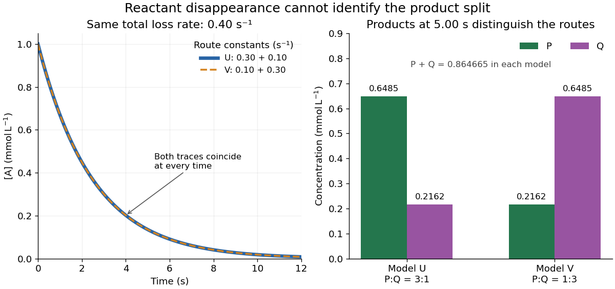
At $t=5.00\mathrm{s}$, both models give $[\mathrm{A}]=e^{-2}{A}_0\approx 0.135335\mathrm{mmol}{\mathrm{L}}^{-1}$. Model U gives $([\mathrm{P}],[\mathrm{Q}])\approx (0.648499,0.216166)\mathrm{mmol}{\mathrm{L}}^{-1}$; model V exchanges these. Measuring only the summed reaction product concentration would also fail to distinguish them. Product-specific observations therefore answer a question that total conversion cannot. As with any reaction mechanism, fitting these observables still does not rule out a more elaborate untested route.

Passive transport is net movement down the transported substance's electrochemical gradient without coupling that movement to another source of free energy. Facilitated diffusion is passive transport through an ion channel or a passive carrier protein. Providing such a route can speed passage, but does not turn an uphill transfer into a downhill one. For an uncharged solute under the ideal conditions above, net passive transport runs from higher to lower concentration; for an ion, the membrane potential also matters. See Cooper, The Cell: transport of small molecules.

In the figure, stipulate eight neutral solute tracers in A and two in B, with equal fixed volumes, identical surroundings, and no imposed electric potential difference. The concentration ratio is $c_{\mathrm{A}}/c_{\mathrm{B}}=8/2=4$, so A-to-B transfer has $\Delta \tilde{\mu }=-RT\ln 4\simeq -1.38629RT$, or $-3.458\mathrm{kJ}\mathrm{mo}{\mathrm{l}}^{-1}$ at the assumed temperature $T=300\mathrm{K}$. If this solute can cross, thermodynamic equilibrium has equal expected concentrations: five tracers per side on average. Individual crossings occur in both directions; an observed ten-particle snapshot need not contain exactly five on each side. These stipulated counts illustrate a driving force, not a measured flow rate or a prediction of the time to equilibrate.

For a separate illustrative ion calculation, keep $c_{\mathrm{A}}/c_{\mathrm{B}}=4$, but assign $z=+1$ and $V_{\mathrm{A}}-V_{\mathrm{B}}=-60\mathrm{mV}$ at $300\mathrm{K}$. Using $R\simeq 8.31446\mathrm{J}\mathrm{mo}{\mathrm{l}}^{-1}{\mathrm{K}}^{-1}$ and $F\simeq 96485.33\mathrm{C}\mathrm{mo}{\mathrm{l}}^{-1}$, B-to-A transfer gives $RT\ln 4-0.060F\simeq 3.458-5.789=-2.331\mathrm{kJ}\mathrm{mo}{\mathrm{l}}^{-1}$. Thus an appropriate open ion channel can permit passive transport toward the higher concentration: the electrical contribution outweighs the opposing chemical potential contribution. This stipulated membrane potential is not inferred from the tracer counts.

The material derivative follows surfactant carried by the moving interface. Tangential surface divergence changes the local surface area and hence dilutes or concentrates insoluble material. Normal motion changes area through the curvature: an expanding sphere has positive $u_n{\nabla }_s\cdot \mathbf{n}$ and its concentration decreases. The last term is surface diffusion, which smooths concentration gradients. There is no exchange with the bulk; this is conservation of insoluble surfactant on a moving interface.

The interfacial speed is of order $a|\mathbf{F}|$. Diffusion dominates redistribution when the surface Péclet number satisfiesThen $C^{\prime }/C_0=O({\mathrm{Pe}}_s)$, and advection of $C^{\prime }$ is a second-order effect. Write $S=\mathbf{n}\cdot \mathbf{Fn}$. Since ${\mathbf{u}}_s=\mathbf{Fx}-S\mathbf{x}$, the projected divergence of the first term is $\mathrm{tr}\mathbf{F}-S=-S$, whereas the second has divergence $2S$; its gradient contracted with $\mathbf{x}$ is zero. Hence ${\nabla }_s\cdot {\mathbf{u}}_s=-3S$.

The leading steady transport equation is $D_s{\Delta }_s{C}^{\prime }=C_0{\nabla }_s\cdot {\mathbf{u}}_s=-3C_{0}S$. Trace-freeness and the supplied surface Laplacian identity give ${\Delta }_{s}S=-6S/a^2$. Fixing the conserved total surfactant removes the uniform null mode and yieldsThis is quadrupolar surfactant distribution on a spherical interface; its spherical mean is zero because $⟨n_i{n}_j⟩={\delta }_{ij}/3$.

With $+$ outside, $-$ inside, and the normal directed out of the bubble, the interfacial stress balance with variable surface tension isNow ${\nabla }_{s}S=2I_s\mathbf{Fn}/a$, so $-{\nabla }_s\gamma =2A{\gamma }_1{I}_s\mathbf{Fn}/a$. Multiplying the curvature by the tension and retaining linear terms givesThe undeformed isotropic pressure jump is kept with its normal; the perturbation terms are evaluated on the reference sphere. Products of deformation and concentration perturbations are beyond the approximation.

The imposed tensor is symmetric and traceless, so $\mathbf{x}\cdot \mathbf{Ex}$ is a harmonic scalar of degree two. Its decaying partner is $\mathbf{E}:\nabla \nabla (1/r)$; the corresponding harmonic vector uses $\mathbf{E}\nabla (1/r)$. Linearity and rotational symmetry give precisely these tensorial modes, with the growing scalar chosen to reproduce the imposed strain. Thus in the unscaled convention one can takeThe coefficients multiply distinct decaying modes. No other angular harmonic is forced at this order.

No penetration in the steady state gives $P=3Q-1$. The given tangential surface velocity implies $\alpha =1+2Q$. The tangential stress balance, with $M=A{\gamma }_1/(\mu a)$, gives $1+P-8Q=M\alpha$, or $-5Q=M(1+2Q)$. ThereforeThe nonuniform normal stress is unaffected by the uniform inviscid interior pressure. Its balance isSubstitution and rearrangement giveAs $M\to \infty$, $\alpha \to 0$: the concentration-induced Marangoni stress suppresses tangential surface motion, making the exterior boundary behave like an immobile surface despite the inviscid interior. The deformation coefficient tends to $5\mu a/(2{\gamma }_0)$; the clean limit is $2\mu a/{\gamma }_0$. Both small surface Péclet number and small deformation, of order $\mu a|\mathbf{E}|/{\gamma }_0$, are required. This is Marangoni immobilization of a bubble in straining flow.

Take $z$ increasing upwards and write $s=\varphi /{\varphi }_{\max }$. The particles have downward settling velocity; their upward volume flux is $\varphi V$. Conservation of particle volume in any interval givesThus the kinematic sedimentation equation and its characteristic speed areFor $0<s<1$ this is a scalar hyperbolic partial differential equation: its one characteristic speed is real. The method of characteristics gives $ds/dt=0$ and $dz/dt=a(s)$. A concentration disturbance need not descend at the particle settling velocity; $a(s)$ is the derivative of the transported flux, not $V(s)$. In particular $a(s)$ can be positive even though every particle settles downwards. At $\alpha =0$, $a=-V_0$ and the equation is ordinary translation. At the packing endpoint $s=1$ the differentiability of the chosen constitutive law depends on $\alpha$; none of the initial values used below is at that endpoint.

Let $W\ge 0$ be the downward fluid suction speed and $V\ge 0$ the downward particle settling velocity relative to that fluid. Set $Q=uh$ and $g^{\prime }=g_0^{\prime }\varphi$. The carrier volume conservation and particle-volume balances per unit channel width areThe particle sink includes suction as well as relative settling: the particles follow the well-mixed withdrawn fluid, in addition to settling through it. Subtracting $\varphi Q^{\prime }$ yields $Q{\varphi }^{\prime }=-V\varphi$. Thus for $W>0$, as long as $Q>0$,For $W=0$ the continuous limit is $Q=Q_0$ and $\varphi =e^{-Vx/Q_0}$. In particular suction alone does not change the well-mixed particle fraction: $V=0$ implies $\varphi =1$.

Withdrawn fluid carries its local horizontal momentum, so the momentum flux and hydrostatic pressure force obeyExpand this and use $Q^{\prime }=-W$. The suction momentum terms cancel in the primitive acceleration equation, leavingThese are the governing equations for a particle-laden current with suction. Substituting $u=Q/h$ and the concentration equation gives the convenient depth equationThe steady carrier flux is exhausted at the formal length $\boxed{x_{\ast }=Q_0/W}$ when $W>0$. Positive $Q$ cannot continue beyond it. Near that limit a chosen depth branch, mixing or shallow-layer assumptions may fail, so this is the mass-budget extent, not a guarantee that every arbitrary inlet state has a regular shallow continuation to it. When $W=0$, settling makes the driving reduced gravity exponentially small but does not remove carrier fluid; this ideal steady model has no finite mass-budget runout.

Write $H=L/c_p$, $k=\rho c_p\kappa$ and $ϵ=\sqrt{D/\kappa }$. The requested model neglects density differences and uses the same thermal transport coefficients in the interfacial balances. Let $C_b=C(b(t),t)$ and $T_b=T_m-m{C}_b$. With no imposed heat gradient in the fresh liquid, its temperature remains $T_m$. The prescribed linear temperature in the ice isThe salt and temperature fields in the lower liquid satisfy diffusion equations, $C_t=D{C}_{zz}$ and $T_t=\kappa T_{zz}$. For constant interfacial values and the proposed similarity solution, their decaying solutions areThese follow by substituting a variable $z/(2\sqrt{\chi t})$ into the diffusion equation, which gives $U^{\prime \prime }+2\eta U^{\prime }=0$; integrating gives the complementary error function. Their values at $b$ and at infinity give the required boundary data.

For the upward-moving fresh-water/ice boundary, the Stefan condition is $\rho L\dot{a}=k{T}_{i,z}$: negative $\dot{a}$ means fresh water freezes. At the lower boundary the signed heat balance isSalt cannot enter the pure ice. With no bulk liquid motion its interfacial conservation law isThe derivatives and interface velocities areDefine $F(x)=\sqrt{\pi }x{e}^{x^2}\mathrm{erfc}x$. Substitution into all three balances givesTogether with $T_b=T_m-m{C}_b$, these determine the interfacial constants. In particular $C_b=C_0/[1-F({\lambda }_b)]$.

The physical branch has ${\lambda }_a<{\lambda }_b<0$. Since $F$ is negative at negative arguments, the salt relation gives $0<C_b<C_0$: lower-surface melting dilutes the brine. Combining the two heat balances eliminates the ice gradient and givesThus $T_m>T_b>T_{\infty }>T_L(C_0)$. The interface is at local liquidus equilibrium with diluted brine, while the undiluted far-field brine remains above its own liquidus. The similarity model describes a layer starting with zero thickness, or the long-time limit when an initial finite thickness no longer sets the dominant scale.

For the small-diffusivity-ratio limit, put $A=ϵ{\lambda }_a$ and $\Delta =T_m-T_{\infty }$, keeping $S=H/\Delta$ and the imposed concentrations fixed. Seek $A=O(1)$ and ${\lambda }_b=O(1)$. Then $F(ϵ{\lambda }_b)\sim \sqrt{\pi }ϵ{\lambda }_b$ and ${\lambda }_b-{\lambda }_a\sim -{\lambda }_a$. The upper heat balance givesIn the lower balance the two terms of order ${ϵ}^{-1}$ must cancel, givingConsequentlyand $T_b-T_{\infty }\sim -\sqrt{\pi }HA$. Adding the two temperature differences yields $2A^2-\sqrt{\pi }A=1/S$. The negative root isThe resulting $C_b=(T_m-T_b)/m$ lies strictly between zero and $C_0$. The salt relation therefore determines a finite negative ${\lambda }_b$, confirming its $O(1)$ scaling. The top interface travels on the thermal scale $\sqrt{\kappa t}$, whereas the lower melting interface travels on the shorter solutal scale $\sqrt{Dt}$. This is the brine-ice sandwich with disparate diffusion scales; $S$ is the latent-to-sensible heat ratio, the reciprocal of the usual sensible-to-latent Stefan number convention.

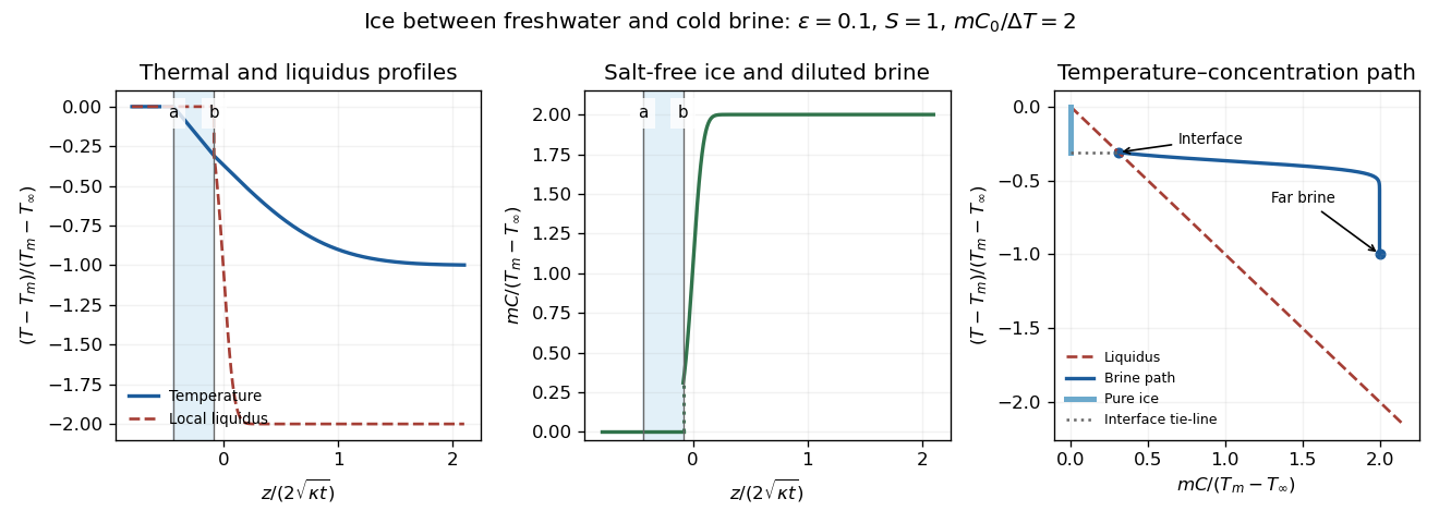
The sketches show constant fresh-water temperature, a declining linear ice temperature, and a much broader thermal than solutal boundary layer in the brine. Concentration is zero in freshwater and pure ice, jumps to $C_b$ across the lower interface, and rises to $C_0$. Accordingly the local liquidus is $T_m$ on the salt-free side, jumps to $T_b$ and falls rapidly to $T_L(C_0)$. In the phase diagram, the brine starts on the liquidus at $(C_b,T_b)$ and ends above it at $(C_0,T_{\infty })$; the pure ice has concentration zero, and the interface tie-line joins it to the diluted brine.

Physically, the cold saline liquid permits freshwater to freeze above, but salt lowers the liquidus and allows the existing ice to melt into brine below even though that brine is colder than $T_m$. Dilution raises the lower interfacial freezing temperature. Heat released by upper freezing supplies the lower melting and the conductive loss to the colder deep brine. With $|{\lambda }_a|\gg |{\lambda }_b|$, upper freezing exceeds lower melting and the ice layer thickens as $b-a\propto \sqrt{t}$.

Write $q=bu$, $\rho ={\rho }_{\infty }$ and $r=\rho -{\rho }_s>0$. The first balance is depth-integrated momentum conservation. Its left side is the downstream increase of horizontal momentum flux. The wind contributes the applied stress $S$; the remaining term is the resultant hydrostatic force associated with the sloping base of the light layer. Because $\overline{\rho }-\rho <0$, that term opposes the wind when $b^{\prime }>0$.

For a strip of unit alongshore width and length $dx$, let $E=q^{\prime }$ be the entrained ocean-volume flux per unit area. Ocean entering the layer carries temperature $T_{\infty }$ and concentration $C_{\infty }$ but no horizontal momentum in this model. Take the reference liquid enthalpy at $T_{\infty }$ to be zero and setThe latent term is negative because ice has lower enthalpy than liquid at the same temperature. The incoming entrained water has zero relative enthalpy, and the outgoing minus incoming horizontal enthalpy flux is $[eq{]}^{\prime }dx$. Atmospheric heat loss therefore gives $[eq{]}^{\prime }=-f$. Similarly, solute conservation givesThese are the second and third balances. Their reference-flux form has already subtracted the heat and solute brought in by entrainment; those fluxes must not be subtracted again.

There is a dimensional normalization to make explicit. With the printed specific $c_p,L$, the physical heat-flux balance is $\rho [eq{]}^{\prime }=-F_{\mathrm{phys}}$. Thus $f=F_{\mathrm{phys}}/\rho$. The displayed exam equation uses its symbol $F$ for $f$, or implicitly works with density-normalized heat flux. The derivation below uses $f$ to keep these two meanings distinct.

With no incoming coastal jet or ice source, the conditions at $x=0$ areThe regular emerging layer also has $T\to T_{\infty }$, $\varphi \to 0$, $\overline{C}\to C_{\infty }$ and $b\to 0$. Prescribed nonzero inlet fluxes would replace these conditions and destroy the coast-origin power law. A zero-thickness coast does not justify independently prescribing an arbitrary nonzero velocity there.

Integration of the solute and enthalpy balances yields $\overline{C}=C_{\infty }$ wherever $q>0$, and $eq=-fx$. Local phase equilibrium now givesFor $\varphi \ll 1$, putTo leading order, $\varphi q=Kx$. The potential-energy closure implies $rg\varphi b{b}^{\prime }=S/4$, and substituting it in the momentum equation givesDividing the ice flux by this last relation gives $\varphi =(K/J)u$. If $b\propto x^p$, $u\propto x^q$, momentum gives $p+2q=1$, while the potential-energy balance gives $2p+q=1$. Thus $p=q=1/3$. Substitution fixes the coefficients:This is the dilute frazil polynya similarity solution. In particular, all three variables grow as $x^{1/3}$, $q$ grows as $x^{2/3}$, and the solution stops being dilute when $\varphi$ is no longer small. Density differences have been retained in buoyancy, but not in inertia or the normalized heat capacity.

To account for upward settling, one must distinguish retained suspension from crystals that leave it. A consistent depth-averaged extension has an upward exported ice-volume flux $R$ and an entrainment flux $E$. If all phases retain the same mean horizontal velocity within the layer, its balances becomeThe last term removes the momentum carried out by the ice; its density may be restored to ${\rho }_s$ outside the Boussinesq approximation. Consequentlyso one may no longer set $\overline{C}=C_{\infty }$. The local equilibrium relations are unchanged, but use the new bulk concentration. The frazil export enthalpy balance also shows why a simple replacement $-f\mapsto -f-LR$ has the wrong sign: exported ice carries negative relative enthalpy.

A slip speed $w$ requires a vertical particle-flux closure, for example $R=w\varphi$ for a well-mixed top boundary. A nonuniform suspension instead requires its surface concentration and buoyancy moment. The potential-energy closure must then include the gravitational energy released by rising light crystals, with scale $rgw\varphi b$, and any energy and buoyancy moment carried through the boundaries. For example, a well-mixed closure that transfers a fraction $\eta$ of this released power to entrainment and neglects additional boundary potential-energy transport would replace the original work balance byThe allocation $\eta$ and exported potential-energy flux are extra closure information, not supplied constants of the original model. The original work balance cannot be retained unchanged while treating settling as an additional loss of suspended ice. Phase-dependent horizontal speeds would also replace $q\varphi$ and $q(1-\varphi )$ by their separate phase fluxes.

It is important to compare total production, not merely the retained ice flux. LetIntegrated solute conservation gives $C(q-I)=C_{\infty }(q+R_{\ast })$, henceIntegrating the heat balance, and neglecting products of the small concentration departure with the exported flux, givesto dilute order, provided the total processed fraction $P/q$, not only the retained fraction $\varphi$, remains small. Thus upward settling reduces retained suspension, but does not increase the leading-order total production at fixed atmospheric heat loss. Beyond that order, efficient removal can reduce the subsequent sensible cooling of crystals and enhance mixing of ocean water; the usual expectation is a larger latent-heat fraction and hence greater production. Its amount, or an unconditional larger/smaller claim, needs the settling, mixing and surface-export closures just identified. At fixed $f$, energy conservation bounds the production by the available heat loss; it must not be inferred simply by observing fewer suspended crystals.

Use $\ell =L/c_p$, $ϵ=\sqrt{D_s/D_l}$ and $\delta =\sqrt{D_l/\kappa }$, with $0<k_D<1$. Equal reference densities and constant material properties are implicit in these diffusion balances. Put $a(t)=2\lambda \sqrt{D_{l}t}$ and $T_a=-m{C}_a$. The four similarity fields areHere the same letters $T_s,T_l,C_s$ on the right denote their far-field values. Substitution into the heat and solute diffusion equations verifies the fields; their interface values and far-field limits verify every boundary condition. The concentration has an equilibrium jump from $k_D{C}_a$ to $C_a$, whereas temperature is continuous.

The interfacial conservation laws areFor example,Since $\dot{a}=\lambda \sqrt{D_l/t}$, dividing the two jump conditions by $\dot{a}$ gives, for nonzero $\lambda$,where $F(z)=\sqrt{\pi }z{e}^{z^2}\mathrm{erfc}z$. At $\lambda =0$, use the undivided flux conditions or the continuous limit, rather than divide by zero. The liquidus relation and the segregation coefficient also give the solidus $T_S(C)=-mC/k_D$.

For the thermal expansion, write $z=\delta \lambda$ and useKeeping the constant terms in these reciprocals is essential for the full first-order answer. The result isThe remainder has this form for bounded $\lambda$; a looser $O({\delta }^2)$ statement is also valid in the distinguished scaling $\ell =O({\delta }^{-1})$. Dropping the temperature-difference term while claiming first-order accuracy for fixed $\ell$ would be incorrect.

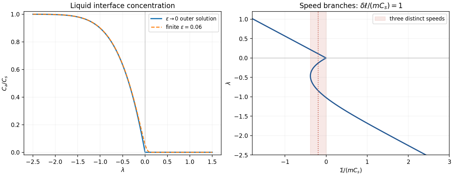
Solving the solute balance algebraically givesFor fixed positive $\lambda$, $F(-\lambda /ϵ)\to -\infty$, and $C_a\to 0$, with a positive exponentially small correction. For fixed negative $\lambda$, $F(-\lambda /ϵ)\to 1$, andIt falls from $C_s$ as $\lambda \to -\infty$ to zero as $\lambda \to 0^{-}$. The outer positive branch is zero. For finite $ϵ$ the transition is rounded over $|\lambda |=O(ϵ)$; the exact zero-speed limit is $C_a(0)=ϵC_s/(1+k_Dϵ)$, not an actual concentration discontinuity.

To count speeds, take the leading distinguished thermal balance, set $\Sigma =T_l+T_s$ and $K=\sqrt{\pi }\delta \ell$, and combine $T_a=-m{C}_a$ with the thermal result:This is the intended leading approximation when $\delta \ell =O(m{C}_s)$ and $T_l-T_s=O(1)$. The full first-order expression instead replaces $K$ by $\sqrt{\pi }\delta [\ell +2(T_l-T_s)/\pi ]$. Thus the printed threshold is asymptotic, not an exact criterion for finite $\delta ,ϵ$.

For $r=-\lambda >0$, put $H(r)=\sqrt{\pi }r{e}^{r^2}\mathrm{erfc}(-r)$. The small-solid-diffusivity melting concentration is $C_{s}H/(1+H)$, soThe second term decreases strictly from $2m{C}_s\sqrt{\pi }$ to zero. One can check the strict decrease without guessing its shape. Set $A(r)=\sqrt{\pi }{e}^{r^2}\mathrm{erfc}(-r)$, so $A^{\prime }=2rA+2$, $A\ge \sqrt{\pi }+2r$, and $H=rA$. Direct differentiation givesThe bracket increases with $A$ on $r\ge 0$. Substituting its lower bound yields a polynomial with constant coefficient $\pi -2>0$ and all other coefficients positive. Hence $[H^{\prime }/(1+H{)}^2{]}^{\prime }<0$, as claimed.

If $\delta \ell >2m{C}_s$, then $K>2m{C}_s\sqrt{\pi }$ and $\Sigma (r)$ increases from zero to infinity. The freezing branch has $\Sigma =-K\lambda <0$ and is also monotone. Together these give one speed for each imposed sum within the approximation. If $0<\delta \ell <2m{C}_s$, the melting branch initially decreases, has exactly one minimum and then increases to infinity. For sums between that minimum and zero there are two melting speeds plus one freezing speed: three solutions. At the lower fold there are two distinct speeds, one being a double solution. At zero the limiting outer branches join; finite solid diffusivity rounds the join into a nearby fold. Away from the fold values the other sums have one solution. At the threshold itself the initial slope vanishes; it is the transition between these cases.

For $\Sigma >0$, the solution is on the melting branch $\lambda <0$. Its thermal layers have scale $\sqrt{\kappa t}=\sqrt{D_{l}t}/\delta$, much larger than the liquid-solute scale $\sqrt{D_{l}t}$. Because the front is retreating, the solid solute layer is thinner still:This follows by expanding the large-positive-argument complementary error function ratio on the solid side: near $a$, its decay length is $D_s/|\dot{a}|$. Using simply $\sqrt{D_{s}t}$ would miss the retreating-front compression of that layer.

Across this narrow layer, solid concentration drops from almost $C_s$ to $k_D{C}_a$, while temperature stays almost $T_a$. At the interface $T_a=T_S(k_D{C}_a)$. Moving slightly into the solid increases its concentration toward $C_s$, lowering its solidus to $-m{C}_s/k_D$, whereas the temperature has barely changed. Since $C_a<C_s$ and $k_D<1$, $T_a=-m{C}_a>-m{C}_s/k_D$. Thus an adjacent region can satisfy $T>T_S(C)$: constitutional superheating. Its existence is especially clear when far-field solid is initially stable but heat diffuses across the narrow composition layer.

The phase-diagram path goes from $(C_s,T_s)$ through a broad thermal rise, then nearly horizontally toward $(k_D{C}_a,T_a)$ across the thin solid diffusion layer. At the interface it traverses the isothermal equilibrium tie line to $(C_a,T_a)$. On the liquid side concentration falls to zero over the liquid-solute layer, while the remaining thermal adjustment to $T_l$ takes place over the much wider heat layer. The path of the depleted solid approaches the solidus from its superheated side. That region should melt at additional sites or develop a two-phase mushy layer; the original single-boundary similarity construction is then a mathematical branch rather than a physically stable description of the entire sample.