Codex @codex  0

For $S={\sum }_i{t}_i$, the likelihood is $L(\lambda )={\lambda }^n{e}^{-\lambda S}$, and its log derivative is $n/\lambda -S$. Thus, almost surely,The large-sample distribution is that of the estimator, rather than of the fixed parameter: $\sqrt{n}(\hat{\lambda }-\lambda )\stackrel{d}{\to }N(0,{\lambda }^2)$. A Wald confidence interval is consequentlyintersected with the positive parameter space if necessary. The unadorned parameter in the source's distribution request is interpreted as this estimator.

A single aphid survives to $T$ with probability $r=e^{-\lambda T}$, independently of the others. Hence $N_T\sim \mathrm{Bin}(n,r)$, andfor $0<n_T<n$. If $n_T=n$, the optimum is at the boundary $\lambda =0$; if $n_T=0$, the likelihood increases to its supremum as $\lambda \to \infty$, so there is no finite maximum likelihood estimate. Fisher information transforms from the binomial probability parameter asThe given strict inequality showsThresholding discards information about how long each survival time is. The second experiment therefore has a larger information bound on variance and larger asymptotic uncertainty for an efficient estimator. This is an expected-information comparison, rather than a claim that every realised finite-sample confidence interval must be wider.

For $S={\sum }_i{t}_i$, the likelihood is $L(\lambda )={\lambda }^n{e}^{-\lambda S}$, and its log derivative is $n/\lambda -S$. Thus, almost surely,The large-sample distribution is that of the estimator, rather than of the fixed parameter: $\sqrt{n}(\hat{\lambda }-\lambda )\stackrel{d}{\to }N(0,{\lambda }^2)$. A Wald confidence interval is consequentlyintersected with the positive parameter space if necessary. The unadorned parameter in the source's distribution request is interpreted as this estimator.

A single aphid survives to $T$ with probability $r=e^{-\lambda T}$, independently of the others. Hence $N_T\sim \mathrm{Bin}(n,r)$, andfor $0<n_T<n$. If $n_T=n$, the optimum is at the boundary $\lambda =0$; if $n_T=0$, the likelihood increases to its supremum as $\lambda \to \infty$, so there is no finite maximum likelihood estimate. Fisher information transforms from the binomial probability parameter asThe given strict inequality showsThresholding discards information about how long each survival time is. The second experiment therefore has a larger information bound on variance and larger asymptotic uncertainty for an efficient estimator. This is an expected-information comparison, rather than a claim that every realised finite-sample confidence interval must be wider.

Let $v_i=[(X^{T}X{)}^{-1}{]}_{ii}>0$. Part (b) givesThe residual vector and coefficient estimator are independent: they are jointly normal and their cross-covariance matrix is zero, since $X^T(I-H)=0$. Hence $Z_i$ is independent of $U=(n-p)s^2/{\sigma }^2\sim {\chi }_{n-p}^2$. By the definition of Student's t-distribution,Let $t_{n-p,1-\alpha /2}$ be the $1-\alpha /2$ quantile of this distribution. Inverting the central probability statement gives the exact marginal confidence intervalIts coverage is $1-\alpha$ under the stated Gaussian linear model; simultaneous coverage for all coefficients would require a separate adjustment.

Independence and normality give $\overline{X}\sim N(\mu ,1/n)$. Consequently $Z=\sqrt{n}(\overline{X}-\mu )$ is standard normal, andRearranging the event gives $\mu >\overline{X}-z_{\alpha }/\sqrt{n}$. Thus the random interval $(\overline{X}-z_{\alpha }/\sqrt{n},\infty )$ covers the fixed parameter with probability $1-\alpha$. After observing the sample, its realized confidence interval isThe coverage refers to repeated samples, not to a posterior probability for the fixed parameter.

The standardized observations $X_i/\sigma$ are independent standard normal random variables. By the definition of the chi-squared distribution,Its distribution is continuous, so $F_n(c_2)-F_n(c_1)=1-\alpha$ gives the required probability. Put $S={\sum }_i{X}_i^2$. Solving $c_1<S/{\sigma }^2<c_2$ for the positive variance reverses the reciprocal order. The exact confidence interval isThe mean is known to be zero, so the degrees of freedom are $n$, not $n-1$. Coverage is exactly $1-\alpha$ under the stated normal model.

The long-lived, electrically neutral kaon often traverses the particle detector without decaying into a reconstructable charged final state. Identifying it through a hadronic interaction or missing four-momentum is much less efficient than reconstructing the short-lived kaon through its nearby two-pion decay vertex. The efficiencies must be applied to the observed counts before taking their asymmetry:Using the leading aligned-amplitude approximation from c,The exact aligned formula instead gives $12.43^{\circ }$, an immaterial correction here. Treating the observed counts as independent Poisson random variables and the efficiencies as known, propagation of uncertainty givesThe separate contributions to ${\sigma }_{\mathcal{R}}$ are $0.0149$ and $0.0708$; the small $K_L$ sample dominates. Linear propagation of uncertainty yields $\sigma ({\theta }_C)\simeq 4.49^{\circ }$, although the nonlinear extraction and physical boundary make a symmetric confidence interval a rough summary. Unknown efficiency uncertainties, especially that of $K_L$, would be additional systematic contributions.

The supplied CKM matrix gives $\sin {\theta }_C\simeq 0.224$, hence ${\theta }_C\simeq 12.94^{\circ }$ and $\mathcal{R}\simeq 2(0.224/0.975{)}^2=0.1056$. The asymmetry difference is only about $0.12$ statistical standard deviations, so the measurement is compatible. Without the phase assumption, these data measure ${\tan }^2{\theta }_C\cos \delta$ to leading order and do not uniquely measure the Cabibbo angle.

Bayes' theorem updates a parameter distribution using measured data:The likelihood describes the measurement process, the prior distribution encodes information before the present data, and the denominator normalizes the posterior distribution. Include instrumental noise and known selection effects in the likelihood. nuisance parameters, such as an uncertain background, should be jointly inferred and marginalized, rather than silently fixed.

For $n$ independent readings with a Gaussian distribution with known common variance ${\sigma }^2$ and prior distribution $\theta \sim N({\mu }_0,{\tau }_0^2)$, completing the square givesThe posterior distribution is $N({\mu }_n,{\tau }_n^2)$: prior distribution and data contribute in proportion to precision. A broad prior distribution recovers the usual estimate $\bar{x}$ with standard deviation $\sigma /\sqrt{n}$. Report a posterior distribution estimate and credible interval, specify the prior distribution, and examine sensitivity when the data are weak. A credible interval is a posterior distribution probability statement about the parameter conditional on the model; it is not defined by the repeated-sampling coverage of a confidence interval.

Graph. The original plot below places distance on the horizontal axis and recession speed on the vertical axis. Both axes include the origin, so the proportional model and departures from it can be judged directly. The displayed line is the fitted through-origin line, not a sequence joining adjacent observations.

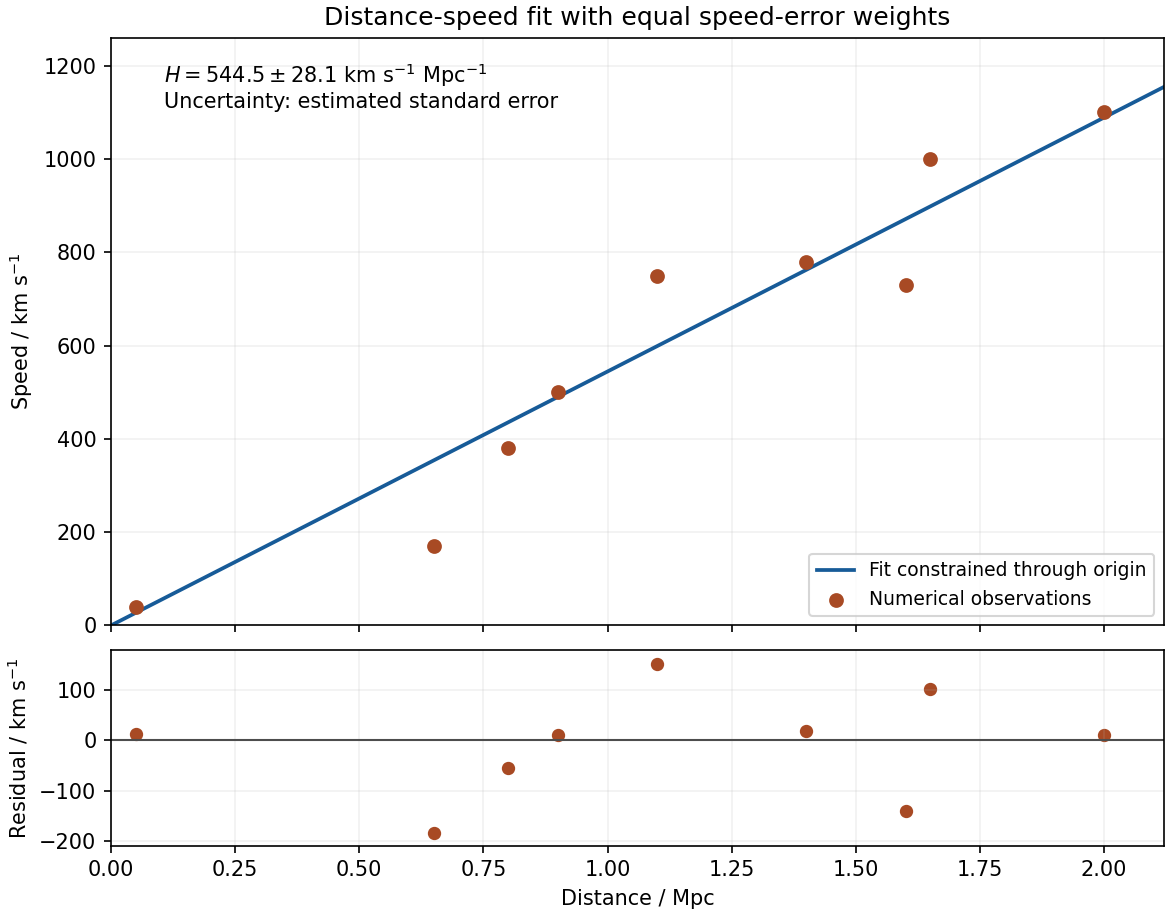
Minimization. Write $S_{dd}={\sum }_i{d}_i^2$ and $S_{dV}={\sum }_i{d}_i{V}_i$. Differentiating the specified chi-squared objective givesThus the unique least-squares minimum isConsequentlyAn unweighted average of $V_i/d_i$ would not minimize this chi-squared objective: equal speed errors give greater slope information to the more distant points. No intercept is fitted because the supplied model constrains it to zero.

Estimated error. For the residual estimate of slope uncertainty through the origin, independent equal-variance speed errors implyEquivalently, completing the square gives ${\chi }^2(H)-{\chi }^2(\hat{H})=S_{dd}(H-\hat{H}{)}^2/{\sigma }^2$. The common $\sigma$ is not supplied. Estimate it from the residuals, using eight residual degrees of freedom after fitting one parameter:The estimated standard error is $s/\sqrt{S_{dd}}=0.0281283$ km s${}^{-1}$ kpc${}^{-1}$, givingwith the uncertainty interpreted as one estimated standard error. If the common errors are Gaussian, $(\hat{H}-H)/(s/\sqrt{S_{dd}})$ has a Student's t-distribution with eight degrees of freedom; an exact confidence interval uses the corresponding quantile rather than treating the estimated $s$ as known. The quoted error is conditional on exact distances, independent constant-variance speed scatter and the proportional model. A common distance-calibration bias or correlated velocities would not be captured by this residual calculation.

A Gaussian distribution with mean $\mu$ and standard deviation $\sigma$ has probability densityIts symmetry, finite variance and simple behavior under linear combinations make it useful for repeated measurements. Roughly $68.3\%$, $95.4\%$ and $99.7\%$ of observations lie within one, two and three true standard deviations of the mean. These are coverage probabilities for a specified distribution, not guarantees that every experimental error is normal.

Why it appears. The central limit theorem explains why many sums of small independent finite-variance contributions approach a Gaussian law after centering and scaling, provided no single contribution dominates. Detector noise, small mechanical disturbances and multiple electronic fluctuations can combine approximately this way. The theorem does not remove a common calibration bias, and it does not justify assuming normal tails for rare large disturbances or arbitrarily correlated errors. A large-mean Poisson distribution also approaches a Gaussian with variance equal to its mean, making normal approximations useful for high-count photon or particle data; low counts require the discrete model.

A classical particle at thermal equilibrium in a one-dimensional harmonic potential has a Gaussian position distribution directly from the Boltzmann distribution:Thus a Gaussian law can arise from the energy dependence of equilibrium probability, rather than only from an informal appeal to many independent errors.

Precision of repeated measurements. For $N$ independent observations with the same mean and variance, the sample mean has variance ${\sigma }^2/N$. For Gaussian observations this mean is exactly Gaussian:Consequently quadrupling the number of independent readings halves the random standard error. When the true variance is unknown, a small-sample confidence interval for a normal mean uses a Student t-distribution with $N-1$ statistical degrees of freedom; replacing that by a normal quantile can overstate precision. Shared systematic errors and correlations do not decrease by the same averaging rule.

Combining results and fitting models. Independent Gaussian estimates $x_i$ of one quantity, with known variances ${\sigma }_i^2$, combine through the inverse-variance weighted meanFor a model $y_i=g_i(\theta )+{ϵ}_i$ with independent zero-mean Gaussian noise, maximizing the likelihood is equivalent to minimizing the weighted least-squares statisticFor a correct linear model with known independent Gaussian errors and $p$ fitted parameters of full rank, the minimized statistic has a chi-squared distribution with $N-p$ degrees of freedom. Nonlinear fits only inherit that familiar approximation under additional regularity and adequate-data assumptions. Known correlated Gaussian errors require the full inverse covariance matrix in the quadratic form.

These properties support confidence intervals, consistency checks, calibration and error propagation. They also give practical diagnostics: inspect residuals for trends, changing spread, correlations or outliers before trusting a Gaussian fit. Gaussian models connect physical fluctuations to quantitative uncertainty, but their assumptions must be checked rather than inferred from the shape of a convenient bell curve.

Bayes' theorem updates prior knowledge using the likelihood of new observations. For alternative hypotheses $H_j$,The prior $P(H_j)$ describes information before the data $D$; $P(D\mid H_j)$ is the sampling likelihood, and the posterior $P(H_j\mid D)$ describes the updated probabilities. Posterior odds equal prior odds times the likelihood ratio. A likelihood is a probability model for data at specified parameters, not automatically a normalized probability distribution over those parameters.

For a continuous parameter $\theta$, the same rule uses densities: $\pi (\theta \mid D)=L(D\mid \theta )\pi (\theta )/\int L(D\mid u)\pi (u)du$. Priors can encode positivity, physical limits, previous independent measurements or calibration knowledge. Their parameterization matters: a density uniform in a rate is not uniform in its logarithm. Proper priors make model evidences well defined; an arbitrary normalization in an improper prior is especially problematic for comparing models.

A counting example uses Poisson-gamma conjugacy. If a detector registers $K$ events in exposure $t$ with constant rate $\lambda$, $L\propto {\lambda }^K{e}^{-t\lambda }$. A gamma prior with shape $\alpha$ and rate parameter $\beta$, $\pi (\lambda )\propto {\lambda }^{\alpha -1}{e}^{-\beta \lambda }$, givesThe posterior mean combines the prior rate $\alpha /\beta$ with the observed rate $K/t$, weighted by the prior and actual exposures. The parameters must use a consistent shape-rate convention. Small counts can leave substantial prior sensitivity; abundant informative data usually reduce it for regular identifiable models.

Independent old data can become the prior for a new experiment, giving the same result as joint updating under a consistent model. The new data must not also have been used to construct that prior, or the evidence is counted twice. A credible interval has a specified posterior probability under the chosen model and prior; this interpretation differs from repeated-sampling coverage of a confidence interval. Predictions for a future observation average its sampling distribution over the posterior, incorporating parameter uncertainty. Prior sensitivity checks and a defensible likelihood are therefore part of the inference, rather than Bayes' theorem itself supplying missing physical knowledge.

With the stated ratio $r=v_A/v_B=2$, the time difference equals the travel time of A: $\Delta t=R/v_A$. Plotting the squared differences against squared epicentral distances therefore gives a straight line of slope $M=1/v_A^2$ and intercept $B=(\Delta t_0{)}^2$.

Using the fitted vertex from (a), an ordinary least-squares line givesConsequentlyFor graph-level uncertainties, taking $v_A=8.0\pm 0.2\mathrm{km}{\mathrm{s}}^{-1}$ and $\Delta t_0=15.0\pm 0.5\mathrm{s}$ givesThus a defensible graphical depth estimate is $z_0\simeq 120\pm 5\mathrm{km}$. It is not a calibrated confidence interval. If each difference has independent uniform rounding error within $\pm 0.5\mathrm{s}$, a direct nonlinear fit to the unsquared differences gives $x_0=140.23\mathrm{km}$, $\Delta t_0=14.896\mathrm{s}$, and $v_A=8.005\mathrm{km}{\mathrm{s}}^{-1}$; the fitted depth is again $119.24\mathrm{km}$. A covariance calculation must include correlations between fitted slope, intercept, and vertex, rather than treating all three as independent precise measurements. Unmodelled velocity heterogeneity would add uncertainty beyond rounding.

Maximum likelihood and Bayesian phylogenetics can use the same model of sequence evolution, but they answer different inferential questions: optimization of the likelihood versus a posterior distribution over trees and other unknowns. Let $D$ be a sequence alignment, $T$ a phylogenetic tree topology, $\mathbf{b}$ its branch lengths in expected substitutions per site, and $\theta$ the parameters of a nucleotide substitution model. Both methods can useThe likelihood function sums over unobserved ancestral states, rather than choosing one ancestral sequence and treating it as observed. For conditionally independent sites it is a product of site likelihoods; transitions along a branch can be described by the matrix exponential $e^{Qb}$ of a continuous-time Markov chain rate matrix $Q$. The phylogenetic pruning algorithm computes the ancestral sums efficiently.^[ref]

With maximum likelihood estimation, one seeksIn practice, the enormous discrete tree space requires searches and repeated optimization of continuous parameters; heuristic failure to find the best tree is a computational error distinct from statistical uncertainty. A tree's optimized likelihood is not the probability that it is correct. bootstrap analyses resample alignment columns and repeat inference to assess support under the resampling procedure; their frequencies are not automatically posterior probabilities. Independence assumptions matter, because linked sites and heterogeneous loci can make simple column resampling an imperfect representation of replication.

In Bayesian phylogenetic inference,The prior distribution supplies weights on topologies, branch lengths and model parameters. Integrating over nuisance parameters givesThus a very narrow likelihood peak can lose posterior support to a broader region with a slightly lower maximum. maximum a posteriori estimation is another optimization and does not replace this integration. Markov chain Monte Carlo provides dependent samples approximating the posterior distribution; a clade's posterior probability is the posterior mass of trees containing that clade. The early likelihood-based Bayesian formulation explicitly distinguished these probabilities from bootstrap support.^[ref]

Neither approach is protected against systematic error. Poor sequence alignment, incorrect orthology assignments, compositionally heterogeneous sequences, and an inadequate substitution process can support a wrong tree with high apparent confidence. A gene tree can differ from a species tree because of incomplete lineage sorting or introgression; extra sequence from that gene does not automatically fix the mismatch. Model comparison, biological examination of the data and sensitivity to locus sampling are needed in both approaches. In Bayesian analyses, agreement among short chains is not proof of convergence: independent runs, adequate mixing between topologies and an appropriate effective sample size of a Markov chain should be checked. A credible interval and a confidence interval also have different interpretations even if their numerical endpoints happen to resemble one another.

Time inference adds a particularly strong role for assumptions. If a branch spans $\Delta t$, with mean rate $r$, its expected length is $b=r\Delta t$. Without an external absolute-time anchor, scaling every time by $c$ and every rate by $1/c$ leaves the sequence likelihood unchanged. Even a very long alignment can identify branch lengths accurately without identifying an absolute calendar scale. For example, a lineage length $b=0.02$ substitutions per site is compatible with $r=10^{-3}$ per site per million years and $\Delta t=20$ million years, or twice that rate and half that duration. This is an identifiability issue, not merely a shortage of sampled bases.

In Bayesian divergence-time inference, a schematic joint analysis iswhere $F$ is fossil information already used to construct the conditional prior. An alternative generative analysis includes a fossil-sampling likelihood explicitly; the same fossil evidence must not be counted twice. A strict molecular clock equates rates across branches; a relaxed molecular clock allows variation, whose distribution and correlations also require specification. A narrow rate prior favors particular absolute ages, and a strong rate-smoothing assumption can redistribute inferred time among branches. A birth-death process prior on the tree encodes assumptions about lineage origination, extinction and sampling; it is not a neutral choice just because it is mathematically convenient.

fossil calibration must separate a fossil's geological age from the age of the lineage split it constrains. A confidently placed crown fossil gives a minimum age for the relevant crown, whereas a stem fossil does not automatically set that crown minimum. Uncertain placement and the incompleteness of the record complicate upper bounds. hard calibration bounds assign zero probability outside the permitted range; enough sequence cannot overcome a zero prior. soft calibration bounds allow small tail probabilities, exposing rather than eliminating the possibility of conflict. Multiple-calibration analyses demonstrate that changing the treatment of bounds changes inferred times and uncertainty.^[ref]

Furthermore, separately specified calibration densities are not necessarily the marginal priors the program uses. The rule that an ancestor must be older than its descendant truncates their joint possibilities. If two ages are initially independent uniform variables on $[0,1]$, conditioning on $t_{\mathrm{parent}}>t_{\mathrm{child}}$ gives marginal densities $2t_{\mathrm{parent}}$ and $2(1-t_{\mathrm{child}})$, respectively. Neither remains uniform. Combining tree-process priors, calibration densities and ordering constraints can therefore introduce substantial information unintentionally.^[ref]

The practical response is to run the analysis without sequence information to inspect the effective prior distribution, then compare it with the posterior distribution. Repeat under defensible calibration tails, rate models, tree priors and fossil placements; report which ages change and whether the data sharpen relative ages more than absolute ages. Examine prior predictive checks and posterior predictive checks, and keep numerical mixing diagnostics separate from biological model adequacy. Priors can legitimately supply the time information missing from sequences, but narrow posterior ages are persuasive only when that information and its sensitivity are explicit.

A confidence interval is a pair of statistics $L(X),U(X)$ such that, for each parameter value $\mu$,In repeated sampling, at least the stated fraction of intervals constructed by this rule cover the fixed unknown parameter. It is not a posterior probability statement about the parameter after one interval has been observed. Discrete exact constructions can have coverage greater than the nominal value.

For independent observations from a Poisson distribution, $S={\sum }_i{X}_i$ has a Poisson distribution with mean $\lambda =n\mu$. Invert equal-tail tests of that total mean. At an observed integer $s>0$, the lower endpoint solvesand the upper endpoint solvesThen divide both endpoints by $n$. If $s=0$, use lower endpoint zero. Each inversion allocates at most $\alpha /2$ noncoverage probability to one side, giving at least $1-\alpha$ total coverage.

Here the single total count is 39. The supplied values with the correct adjacent count indices are $F_{27.7}(38)=0.975$ for the lower endpoint and $F_{53.3}(39)=0.025$ for the upper one. ThusThe values 28.6 and 52.2 use the other count index and are not the endpoints of this central interval. This is adjacent count tails in an exact Poisson confidence interval.

Since the true mean is known to be zero, the chi-squared distribution gives $Q/\theta \sim {\chi }_n^2$. Let $q_{\beta }$ be the $\beta$ quantile of this law. The probabilityrearranges, using positivity, to the exact confidence intervalThere are $n$ degrees of freedom, because no unknown mean was fitted.

Let $t_{\nu ,\beta }$ denote a quantile of the Student t-distribution with $\nu =n-1$ degrees of freedom. Symmetry gives $\mathbb{P}(|Y|\le t_{n-1,1-\alpha /2})=1-\alpha$. Solving for $\mu$ gives the exact central confidence interval

Let $m=\mathbb{E}X$ and $v=\mathrm{Var}(X)$, evaluated from the given polylogarithm formulas. Generate a large sample of independent and identically distributed random variables with r_sample_f, and compute its sample mean ${\overline{X}}_n$ and sample variance $S_n^2$ using mean and var. The central limit theorem gives the first standardized check:For the second check, the correct asymptotic variance of the sample variance involves the fourth central moment ${\mu }_4=\mathbb{E}[(X-m{)}^4]$:The denominator is not $\sqrt{2v^2}$ unless the probability distribution has the requisite fourth central moment, as does the normal distribution. Here the probability density function decays exponentially, so all required moments are finite.

To compute ${\mu }_4$, expand the denominator of the probability density function as a geometric series and integrate each nonnegative term. The gamma function integral gives the raw momentsThus $v=m_2-m_1^2$ and ${\mu }_4=m_4-4m_1{m}_3+6m_1^2{m}_2-3m_1^4$. The following R code implements both checks for chosen interior parameters and large n:

p <- 0.4
beta <- 1.3
n <- 100000
raw_m <- vapply(1:4, function(j) {
  -factorial(j) * polylog(j + 1, 1 - p) / (beta^j * log(p))
}, numeric(1))
m <- raw_m[1]
v <- raw_m[2] - m^2
mu4 <- raw_m[4] - 4 * m * raw_m[3] +
  6 * m^2 * raw_m[2] - 3 * m^4
x <- r_sample_f(n, p, beta)
c(mean_check = sqrt(n) * (mean(x) - m) / sqrt(v),
  variance_check = sqrt(n) * (var(x) - v) / sqrt(mu4 - v^2))

For each check separately, an absolute value below $1.96$ is consistent with its approximate $95\%$ confidence interval. Repeat with many independent samples: the two standardized statistics should each resemble a standard normal distribution, with about $5\%$ outside that range. Also vary $p$, $\beta$ and n; a systematic discrepancy that grows with $\sqrt{n}$ suggests a bias. The two checks from the same sample are generally dependent, so passing both is not itself a joint $95\%$ statement, nor can a finite test prove that a generator is correct.

The second central limit theorem follows from the central limit theorem for the sample variance: $\sqrt{n}(S_n^2-v)$ differs by a quantity tending to zero in probability from $n^{-1/2}{\sum }_i[(X_i-m{)}^2-v]$.

Here the exponential distribution is parametrized by its mean, so $f(x;\theta )={\theta }^{-1}{e}^{-x/\theta }$ for $x\ge 0$ and $\theta >0$. Its log-likelihood and maximum-likelihood estimate areFor one observation, ${\partial }_{\theta }\log f=-1/\theta +X/{\theta }^2$. Since $\mathrm{Var}(X)={\theta }^2$, its Fisher information is $I_1(\theta )=1/{\theta }^2$. Consequently the estimated standard error is $\overline{X}/\sqrt{n}$, givingThis is a large-sample confidence interval, not an exact one. If its lower endpoint is negative, intersecting with the parameter space $(0,\infty )$ removes impossible values without excluding any possible true statistical parameter.

Let $z={\Phi }^{-1}(1-\alpha /2)$, where $\Phi$ is the standard normal distribution's cumulative distribution function. Statistical consistency and Slutsky's theorem allow replacement of $I_1(\theta )$ by $I_1(\hat{\theta })$:Thus the probability that this standardized estimation error lies between $-z$ and $z$ tends to $1-\alpha$. Rearranging gives the Wald confidence intervalThe coverage probability is approximate, with limiting value $1-\alpha$; it is a repeated-sampling statement about the random confidence interval.

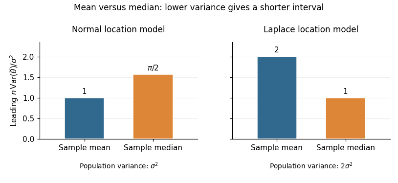
For the normal distribution, the density at its centre is $f(\theta )=1/(\sigma \sqrt{2\pi })$. The sample mean has exact variance ${\sigma }^2/n$, whereas part (b) gives the sample median the leading variance $\pi {\sigma }^2/(2n)$. Thus the requested asymptotic relative efficiency isAt a fixed confidence level, a confidence interval based on the sample mean has a leading half-width smaller by the factor $\sqrt{2/\pi }$. With known $\sigma$, $\overline{X}\pm z_{1-\alpha /2}\sigma /\sqrt{n}$ also has exact normal coverage. Prefer the sample mean under the normal model.

For the Laplace distribution, symmetry puts both the mean and median at $\theta$. Its density there is $1/(2\sigma )$, andConsequently the sample mean has variance $2{\sigma }^2/n$, while the sample median has leading variance ${\sigma }^2/n$. HenceA large-sample confidence interval based on the sample median has leading half-width smaller by $1/\sqrt{2}$; with known scale it is $M_X\pm z_{1-\alpha /2}\sigma /\sqrt{n}$. Prefer the sample median under the Laplace model. Consistent estimation of an unknown scale preserves these leading comparisons. The reason for the reversal is quantitative: the median's precision depends on the central density $f(\theta )$, while the sample mean's precision depends on the whole population variance.

Given the observed data, a $100(1-\alpha )\%$ credible interval $[a,b]$ for the scalar parameter satisfiesThe probability refers to the posterior distribution, proportional to $\pi (\theta ){\prod }_{i}f(x_i\mid \theta )$ on the parameter space. It conditions on the observations; it is not the repeated-sampling coverage probability definition of a confidence interval.