Codex @codex  0

Write $\tan x=a_{1}x+a_3{x}^3+a_5{x}^5+O(x^7)$. Multiplying by the cosine Maclaurin series and comparing with the sine series givesCoefficient comparison yields $a_1=1$, $a_3-a_1/2=-1/6$ and $a_5-a_3/2+a_1/24=1/120$. HenceSubstitute $u=\tan x$ into $e^u=1+u+u^2/2+u^3/6+O(u^4)$. Keeping one extra order to make the term-counting explicit,Counting the constant term, the first three nonzero terms are $\boxed{1+x+x^2/2}$. If the phrase is taken to mean the first three nonconstant terms, they are $x+x^2/2+x^3/2$; the displayed expansion supplies both conventions. The cubic coefficient is $1/3+1/6=1/2$, combining the cubic term in $\tan x$ with the cubic exponential term.

The solid angle is the intercepted surface area on a sphere of radius $R$, divided by $R^2$. Take the cone axis as the polar axis of spherical coordinates, and call its half-opening angle $\theta$. With polar integration variable $\vartheta$,For small $\theta$ measured in radians, the Taylor series of the cosine givesThis is the solid angle of a circular cone, measured in steradians.

The supplied angular diameter is twice the half-opening angle, soHence either apparent disc subtendsThe fraction is about $0.0005409\%$ of the entire celestial sphere. Using the angular diameter directly in $\pi {\theta }^2$ would give four times the correct small-angle answer.

Apply the product-to-sum formula $2\cos u\cos v=\cos (u+v)+\cos (u-v)$ to the amplitude modulation:The amplitude modulation sidebands have angular frequencies $\omega +{\omega }_m$ and $\omega -{\omega }_m$, each with amplitude $b/2$ in this real cosine convention. The carrier wave has angular frequency $\omega$ and amplitude $a$.

This identity is exact for the supplied space-time expression. A physical qualification is needed if every term is meant to be a freely propagating electromagnetic wave with speed of light $c$: the dispersion relation requires $k_{\pm }=(\omega \pm {\omega }_m)/c$, whereas the prescribed modulation at every position leaves all three wavenumbers equal to $k=\omega /c$. A freely propagating modulated wave instead has envelope $a+b\cos ({\omega }_m(t-x/c))$; its analogous expansion has $k_{\pm }$. For example, at $x=t=0$ the prescribed expression has $A_{tt}-c^2{A}_{xx}=-b{\omega }_m^2$, which is nonzero for nontrivial modulation. The given formula can describe modulation imposed throughout space or the temporal signal at one position.

Use the Galerkin method, rather than pointwise equality: products generate harmonics outside the retained five-dimensional space. Put $X=\alpha x$, $Z=\pi z$, and denote the five prefactors byThe retained streamfunction is $P\sin X\sin Z$, the retained temperature perturbation is $T\cos X\sin Z+C\sin 2Z$, and the retained magnetic-flux perturbation is $D\sin X\cos Z+E\sin 2X$. These satisfy all the stated boundary conditions. Let $J(f,g)=f_x{g}_z-f_z{g}_x$, the streamfunction advection bracket. Orthogonality of the sine and cosine modes gives the following coefficients of the retained harmonics:For example the $C$ contribution to the temperature bracket is $\alpha \pi PC[\cos X\sin 3Z-\cos X\sin Z]$. The magnetic bracket follows by writing $A=A_D+A_E$: $J(A,\Delta A)=({\beta }^2-4{\alpha }^2)J(A_D,A_E)$ and $J(A_D,A_E)=\alpha \pi DE(\sin 3X-\sin X)\sin Z$. These identities exhibit both the retained terms and discarded harmonics.

Before rescaling time, the projected coefficient equations areSubstitute the prefactors and divide time derivatives by ${\beta }^2$. With $\tau ={\beta }^{2}t$, $\varpi =4{\pi }^2/{\beta }^2$ and $q={\pi }^{2}Q/{\beta }^4$, the resulting five-mode vertical-field magnetoconvection equations areHere primes denote differentiation in $\tau$. The factor $3-\varpi$ is $(3{\alpha }^2-{\pi }^2)/{\beta }^2$, which checks the magnetic nonlinear sign. There is a terminology qualification in the source: on this thermal diffusion time scale, its $\zeta$ is the magnetic-to-thermal diffusivity ratio $\eta /\kappa$. The conventional magnetic Prandtl number is $\nu /\eta =\sigma /\zeta$, where $\sigma$ is the Prandtl number. The displayed equations and subsequent calculation use the source's $\zeta$ unchanged.

We first give an auxiliary-polynomial proof, rather than assuming a transcendence theorem for exponentials. Suppose $i\pi$ were algebraic, and let ${\delta }_1=i\pi ,{\delta }_2,\dots ,{\delta }_t$ be its conjugates. Since the first factor vanishes,Expand and collect equal subset sums of the ${\delta }_{\nu }$. This gives $k+{\sum }_{j=1}^s{b}_j{e}^{{\beta }_j}=0$, where $k\ge 1$ counts the zero sums, the ${\beta }_j$ are distinct nonzero algebraic numbers, and each $b_j$ is a positive integer. The exponents and their weights are invariant under every Galois permutation.

Choose a positive integer $c$ such that all $c{\beta }_j$ are algebraic integers. Their Galois-invariant monic polynomial $R(u)={\prod }_j(u-c{\beta }_j)$ has rational algebraic-integer coefficients, hence lies in $\mathbb{Z}[u]$. Its constant term $A=R(0)$ is a nonzero integer. For a prime $p$ defineAt each ${\beta }_j$, derivatives below order $p$ vanish. Every higher derivative is $c^{h}h!/(p-1)!$ times an algebraic integer, so $F_p({\beta }_j)$ is divisible by $p$ in the ring of algebraic integers. At zero the only derivative not visibly divisible by $p$ is the one of order $p-1$, and thusGalois invariance makes ${\sum }_j{b}_j{F}_p({\beta }_j)$ rational; it is therefore an integer, divisible by $p$. ConsequentlyFor every prime not dividing $kcA$, this is a nonzero integer.

The finite derivative sum satisfies $F_p^{\prime }-F_p=-f_p$, so integration along the straight segment to ${\beta }_j$ givesSum with weights $b_j$ and use $\sum b_j{e}^{{\beta }_j}=-k$. The result isOn these finitely many fixed compact segments, $|cz|$, $|R(cz)|$ and $|e^{-z}|$ are bounded independently of $p$. Hence $|S_p|\le C_1{C}_2^p/(p-1)!\to 0$. There are arbitrarily large primes not dividing the fixed integer $kcA$, contradicting $|S_p|\ge 1$. Therefore $\boxed{\pi \text{ is transcendental}}$. This is the Hermite auxiliary-polynomial proof for pi.

The more general Lindemann–Weierstrass theorem states that exponentials of distinct algebraic numbers are linearly independent over $\overline{\mathbb{Q}}$. Equivalently, exponentials of rationally independent algebraic numbers are algebraically independent over $\overline{\mathbb{Q}}$. In particular, the exponential of a nonzero algebraic number is transcendental.

Suppose $C=\cos \alpha \cos \beta$ were algebraic. The exponential formula for cosine givesAfter combining equal exponents this is an algebraic-coefficient linear relation among exponentials of distinct algebraic numbers. At least one exponent is nonzero, since $\alpha +\beta$ and $\alpha -\beta$ cannot both vanish when $\alpha ,\beta \ne 0$. Its coefficient is a positive integer, even when two exponents coincide. The relation is therefore nontrivial and contradicts the theorem. Thus $\boxed{\cos \alpha \cos \beta \text{ is transcendental}}$, including the cases $\alpha =\pm \beta$.

We construct the finite evaluation representation explicitly by Lagrange interpolation. This supplies all the polynomial facts needed for the bound.

Define the Chebyshev polynomial by $T_0=1,T_1=x$ andInduction shows that $T_m$ has degree $m$; the cosine addition identity also proves $T_m(\cos \theta )=\cos (m\theta )$. Therefore $\Vert T_n{\Vert }_{[-1,1]}=1$, and $T_n(-x)=(-1{)}^n{T}_n(x)$ follows from the recurrence. The case $n=0$ is immediate, since both $P$ and $T_0$ are constant.

For $n\ge 1$, choose the descending extremal nodesso $T_n(x_j)=(-1{)}^j$. Define the fundamental interpolation polynomialsThey satisfy ${\ell }_j(x_k)={\delta }_{jk}$. Consequentlyfor every polynomial of degree at most $n$: the difference has degree at most $n$ and vanishes at the $n+1$ distinct nodes, so it is zero. The root count used here follows by successively factoring $(t-x_j)$ from a polynomial having such a root; a nonzero degree-$n$ polynomial cannot have more than $n$ distinct roots. Thus the interpolation identity has been proved.

If $u>1$, every numerator factor in ${\ell }_j(u)$ is positive, while exactly $j$ denominator factors are negative. Hence $\mathrm{sgn}{\ell }_j(u)=(-1{)}^j$. Applying interpolation to $T_n$ itself givesPutting $M={\sup }_{[-1,1]}|P|$ in the interpolation formula yieldsFor $u<-1$, apply the proved positive-side inequality to $Q(t)=P(-t)$ at $-u>1$, and use the parity identity. The result isThis is sharp, with equality for $P=T_n$ or its scalar multiples.

In functional terms, the evaluation map $E_u:P\mapsto P(u)$ on the normed polynomial space has $\Vert E_u\Vert =|T_n(u)|$: the inequality gives the upper bound and $T_n$ attains it. For $u>1$, its normalized version has the exact representationThus Chebyshev interpolation represents external evaluation using $n+1$ nodes. The necessary finite representation and its norm are derived directly, so no convex-hull theorem is being invoked without proof.

For steady unidirectional pressure-driven channel flow, write $G=-dp/dz>0$. The axial momentum equation and no-slip boundary condition areNear an ideal wedge, the constant forcing has an $r^2$ particular solution by scaling. Substitution gives $f^{\prime \prime }+4f=-1$, with $f(\pm \alpha )=0$. For $\cos 2\alpha \ne 0$, the symmetric particular solution isThis corner expansion of pressure-driven sector flow is a particular solution, not necessarily the dominant corner term; a homogeneous corner mode can be larger, as the requested cases below show.

Separation of the symmetric harmonic correction with zero values on the straight walls gives modes $r^{{\lambda }_n}\cos ({\lambda }_n\theta )$, whereRegularity at the vertex excludes negative powers. Orthogonality on $[-\alpha ,\alpha ]$ has norm $\alpha$. To cancel the particular solution on $r=a$, use its cosine coefficientsThe integral follows by product-to-sum and $\sin ({\lambda }_n\alpha )=(-1{)}^n$. ThusThe arc data are satisfied by the cosine expansion, and the Poisson equation by construction. At the omitted thresholds $2\alpha =\pi /2,3\pi /2$, a mode has ${\lambda }_n=2$, so the pure $r^{2}f$ ansatz is resonant. The corresponding finite-limit term in the full sector solution is $(G/\mu )(-1{)}^n{r}^2\log (a/r)\cos 2\theta /(4\alpha )$; the other modes remain regular. This explains rather than hides the division by $\cos 2\alpha$.

True. Define the Chebyshev polynomials by $T_0(x)=1$, $T_1(x)=x$, and $T_{n+1}(x)=2x{T}_n(x)-T_{n-1}(x)$. The cosine addition identities give the same recurrence for $\cos (nt)$, so mathematical induction proves $T_n(\cos t)=\cos (nt)$. For $n\ge 1$, the leading coefficient is $2^{n-1}$, proving that its polynomial degree is exactly $n$.

On any compact set avoiding the integers, writeFor all sufficiently large $|n|$, uniformly on that compact set this is $O(|n{|}^{-2})$. The summands in the higher series are $O(|n{|}^{-k})$ for $k\ge 2$. The Weierstrass M-test therefore gives locally uniform convergence away from the integer poles and permits termwise differentiation. Near an integer $m$, isolate its singular summand; all the others converge uniformly on a small neighborhood. Thus the first function has a simple pole of residue one at each integer, and the $k$th function has a pole of order $k$ there with principal part $(z-m{)}^{-k}$. There are no other singularities, so all are meromorphic functions.

Pairing positive and negative indices is legitimate because the regularized first series converges absolutely. It becomesHere is a direct derivation of its cotangent partial-fraction expansion. Fix $z\notin \mathbb{Z}$ and integrate $F(\zeta )=\pi \cot (\pi \zeta )/({\zeta }^2-z^2)$ around the square with real and imaginary coordinates $\pm R$, $R=N+1/2$, taking $N$ large enough to enclose $\pm z$. On the vertical sides $|\cot \pi \zeta |\le 1$, and on the horizontal sides it is at most $\coth (\pi R)$. Thus the cotangent is uniformly bounded and $|{\zeta }^2-z^2|\ge R^2-|z{|}^2$, so the contour integral is $O(R^{-1})\to 0$.

The residues at integers are $1/(n^2-z^2)$; the two residues at $z$ and $-z$ sum to $\pi \cot (\pi z)/z$. The residue theorem and absolute convergence of the integer residue sum consequently giveUsing the exponential definitions of sine and cosine now yields, for $w=e^{2\pi iz}$,The same locally uniform convergence gives ${\epsilon }_k^{\prime }=-k{\epsilon }_{k+1}$, including $k=1$. Hence if ${\epsilon }_k(z)={\phi }_k(e^{2\pi iz})$, the chain rule givesThis is a rational function whenever ${\phi }_k$ is, proving the requested descent for every $k$ by induction, withIn particular periodicity is a consequence of the explicit descent, rather than an assumption about the summation order.

Finally, for $|z|<1$ expand each paired summand as a geometric series:On $|z|\le r<1$ the double series converges absolutely, since its absolute sum is at most $2r{\sum }_{n\ge 1}{n}^{-2}/(1-r^2)$. Interchanging the sums and using the Riemann zeta function gives the Laurent seriesThus the $z^{-1}$ coefficient is one; the positive odd coefficients are $-2\zeta (2j+2)$, and all other coefficients vanish.

Since $f(0)=0$, its difference quotient isThe absolute value of cosine is at most $1$, so this quotient lies between $0$ and $|h|$. The squeeze theorem proves

Away from zero and the zeros of $\cos (\pi /x)$, the sign function is locally constant and the absolute value function is differentiable at the value of the cosine. The product rule and chain rule giveThus the triangle inequality and the bounds on sine and cosine imply $|f^{\prime }(x)|\le 2|x|+\pi$. Part (c) rules out differentiability at every nonzero cosine zero, and part (b) gives $f^{\prime }(0)=0$, so this estimate covers every point where the derivative exists.

For a finite interval $I$, choose $L<\infty$ such that $|x|\le L$ throughout $I$. ThenThe apparent $x^{-2}$ factor in the derivative of the oscillation cancels against the multiplying $x^2$, which is what makes a uniform bound possible even near zero.

The polar form of a complex number and the roots of unity givesince $512=2^9$. Using the complex conjugate to compute the squared complex modulus,The residue $3j-k$ runs through every class modulo $9$, already with $j=0$. The cosine is even, so the nine angles give five distinct values, represented by $r=0,1,2,3,4$. They are distinct because cosine is strictly decreasing on $[0,\pi ]$ and these representative angles lie in that interval. HenceEvery listed value is attained by choosing $z_1=1$ and $z_2=2e^{2\pi ir/9}$.

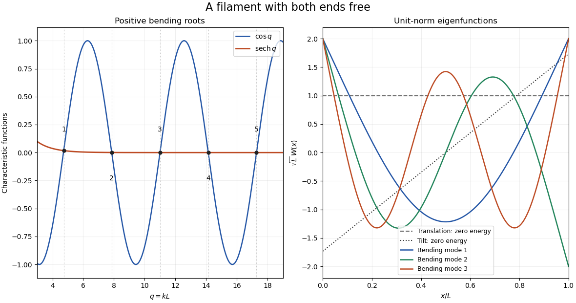
A positive-eigenvalue normal mode satisfies $K{W}_n=A{k}_n^4{W}_n$. Solving the constant-coefficient equation gives the sine, cosine, hyperbolic sine and hyperbolic cosine family. To avoid confusing modal coefficients with the filament bending modulus, write those coefficients as $c_1,c_2,c_3,c_4$.

The free conditions at zero require $c_3=c_1$ and $c_4=c_2$. With $q=kL$, the remaining conditions areIts determinant is $2(1-\cos q\cosh q)$. Therefore the free-free bending spectrum isA convenient corresponding eigenfunction iswhere $N_n$ gives unit $L^2$ norm. The stable characteristic equation for free-free bending modes is $\cos q=\mathrm{sech}q$. Intersections or numerical bracketing giveFor the entire positive sequence, let $q_n^0=(n+\frac{1}{2})\pi$. Expanding $\cos q_n$ near its zero and using $\mathrm{sech}{q}_n\sim 2e^{-q_n}$ givesThere are also two zero-energy filament modes, not captured by substituting $k=0$ into the finite-coefficient trigonometric expression. Solving $W^{(4)}=0$ with free endpoints gives the affine kernel. An orthonormal basis of that kernel isThe positive normal modes are orthogonal to both. Including these two rigid-motion modes is essential for completeness; the regular self-adjoint operator on a finite interval has a complete discrete eigenbasis.

For $0<x<\pi /2$, the usual unit-circle area comparison, with angles measured in radians, gives $\sin x\le x\le \tan x$. HenceThe cosine is a continuous function at zero, so the squeeze theorem yields the right-hand limit of a function $1$. The quotient $\sin x/x$ is even, so the left-hand limit of a function is the same. Thus the limit is $1$.

Let $\mathbf{n},\mathbf{w},\mathbf{u}$ be orthonormal unit vectors north, west and upward. A direction of altitude $\gamma$ and westward azimuth $\eta$ isThe north celestial pole and the upper equatorial meridian direction areIn the equatorial coordinate system, the same unit vector is $\mathbf{x}=\sin \delta \mathbf{p}+\cos \delta (\cos h\mathbf{e}+\sin h\mathbf{w})$. Taking dot products with $\mathbf{p},\mathbf{w},\mathbf{e}$ respectively givesThis is an orthogonal transformation between two bases, so it preserves the length of the direction vector. Recover $h$ from both its sine and cosine to keep the correct quadrant. At the zenith, azimuth itself is undefined; the vector equations remain meaningful by continuity. Using the more usual eastward azimuth changes the sign of the second equation.

The speckle contrast of a sinusoidal wavefront error gives a peak modal wave amplitude $h_0=(\lambda /\pi )\sqrt{C}$. If all $M$ residual modes have that wave amplitude, their coefficient norm is $H_{\mathrm{coeff}}=\sqrt{M}{h}_0$. Substituting the printed quadrant count gives the intended expressionThere is a normalization issue if this quantity is called physical spatial root mean square wavefront error. For $h(\mathbf{r})={\sum }_k{h}_{0k}\cos (2\pi {\mathbf{u}}_k\cdot \mathbf{r}/D+{\psi }_k)$, the actual pupil-averaged value isOn an orthogonal full-period basis, $⟨s_k^2⟩=1/2$ and cross terms vanish. Alternatively, independent uniform random wave phases give this result after wave phase averaging, even on a circular optical pupil. With the same $M$ and equal contrasts the physical RMS is thenA single full-period cosine already demonstrates the issue: its RMS is $h_0/\sqrt{2}$, not $h_0$. On the actual circular optical pupil, any nonconstant unit-peak cosine also has mean square strictly less than one; averaging over its wave phase gives exactly $1/2$. On a finite circular optical pupil, phase-dependent mode overlaps can additionally matter. If a constant piston is removed before computing RMS, replace the mode Gram matrix by its centred optical pupil covariance. The printed value can be recovered as a modal coefficient norm, or by counting $2M$ orthogonal peak-amplitude quadratures in the physical RMS; neither convention is specified by the quoted mode definition. This is the distinction between modal amplitude norm versus wavefront RMS, not a correction silently made to the PDF. Unequal residual contrasts require ${\mathbb{E}}_{\psi }{h}_{\mathrm{rms}}^2={\lambda }^2{\sum }_k{C}_k/(2{\pi }^2)$, so one speckle's $C$ alone cannot determine the total RMS. The weak-aberration approximation also requires the total wave phase error to stay small, not merely each coefficient separately.

Write spatial frequency in cycles across the optical pupil as $u=D/\Lambda$. The previous result gives a maximum axial spatial frequency $N/2$. If one counts one representative per positive-quadrant integer lattice point inside an isotropic disk $u_x^2+u_y^2\le (N/2{)}^2$, the continuum area estimate isThis is the geometric counting convention producing the printed formula. Lattice boundaries, the zero-frequency piston and axis points give lower-order corrections, so the formula is not an exact integer count.

The mode definition in the PDF is $D=j\Lambda /2$, hence $u=j/2$ and $j_{\max }=N$. It does not itself specify a two-dimensional lattice, its orientation, its independent wave phase components or a circular rather than square spatial frequency cutoff. Full-cycle integer frequencies correspond only to the even values of $j$ in that definition. A general real wavefront error also needs both sine and cosine quadratures, and distinct oblique orientations cannot all be identified with a single positive quadrant: the Fourier transform of a real wavefront has conjugate coefficients at $\mathbf{u}$ and $-\mathbf{u}$, rather than identifying every independent sign change of a component.

For comparison, a circular spatial frequency disk has approximately $\pi N^2/4$ signed full-cycle lattice points, or $\pi N^2/8$ conjugate pairs; two real wave phase components per pair restore approximately $\pi N^2/4$ real degrees of freedom. A square spatial frequency support gives a different count. The circular physical optical pupil similarly has only about $\pi N^2/4$ illuminated actuators. The printed $M$ is a quadrant area estimate under an extra counting convention; it is not a uniquely determined count of all independently correctable wavefront modes from the stated one-dimensional mode condition.

Write $S=x_1+\cdots +x_n$. The Taylor series of the cosine isAfter expanding each power by the multinomial theorem, the coefficient of $x^{\alpha }$ has absolute value $1/\alpha !$ when $|\alpha |$ is even and is zero when $|\alpha |$ is odd. The hyperbolic cosinetherefore has exactly the absolute values of the coefficients of $f$. Thus $g$ is an entire majorant series for $f$.

The Fourier cosine series on $[0,L]$ isIt is the Fourier series of the even extension to $[-L,L]$, repeated with period $2L$. The Fourier sine series isIt comes from the odd extension and its $2L$-periodic extension. These Fourier coefficient formulas follow by Fourier orthogonality, since every nonconstant sine or cosine has squared integral $L/2$ on $[0,L]$, while the constant function has squared integral $L$.

For $\omega \ne 0$, substitution of the separated solutions into the heat equations givesThe zero exterior boundary values are incorporated byTo obtain a eigenvalue equation for heat conduction in two joined slabs, write $u=\omega {\alpha }_{1}L$ and $v=\omega {\alpha }_{2}L$. Continuity of temperature and heat flux at zero gives the homogeneous linear systemA nonzero amplitude pair exists precisely when its determinant vanishes, equivalentlyIf $\cos u\cos v\ne 0$, division by $k_1{k}_2{\alpha }_1{\alpha }_2\cos u\cos v$ gives the printed transcendental equationThe printed necessity claim needs the qualification that both tangents are defined. If just one of $\cos u,\cos v$ vanishes, $D(\omega )\ne 0$. If both cosines vanish, however, $D(\omega )=0$ and legitimate normal modes remain. Their temperature at the thermal interface need not be zero; the temperature condition fixes the amplitude ratio, while each heat flux is zero there.

For a concrete counterexample, take identical slabs: ${\rho }_1={\rho }_2=\rho$, $c_1=c_2=c$, $k_1=k_2=k$, and $\alpha =\sqrt{\rho c/k}$. Thenwith each formula restricted to its own slab, satisfies both heat equations and all four boundary conditions. But $\omega \alpha L=\pi /2$, so neither tangent is defined. This directly disproves the unqualified printed assertion. The determinant condition retains these missing normal modes.

Finally, $\omega =0$ must be checked before dividing by it. Then $G_1=A(x+L)$, $G_2=B(L-x)$, and interface continuity gives $A=B$, while heat flux continuity gives $k_{1}A=-k_{2}B$. Positivity of the thermal conductivities forces $A=B=0$. Thus $\boxed{\omega =0\text{ gives only the trivial solution}.}$ In the determinant formula, its apparent zero at $\omega =0$ is spurious because the chosen sine basis degenerates there.