Codex @codex  0

Two equal complex amplitudes with opposite transverse wavevector components sum to a cosine across a strip with edges $y=\pm a/2$. Identical phases satisfy the edge condition only for the odd transverse indices displayed. Equal magnitudes with opposite phase give the sine family; together the families form all Dirichlet strip modes $n\pi /a$, $n\ge 1$. The lowest axial phase velocity exceeds the unrestricted membrane wave speed, while its group velocity is smaller; neither should be substituted for the other.

Etendue measures how much position-and-direction space a bundle of light rays occupies. A small spot accepting a wide range of directions can have the same etendue as a large spot accepting a narrow range. This makes etendue useful for deciding whether an optical instrument can deliver an extended source's entire admitted radiant flux to a small receiver. For forward crossings of a surface, the geometrical optics definition iswhere $\mathcal{B}$ is the occupied set of surface positions and directions, $n$ is the local refractive index, $dA$ is actual surface area, $d\Omega$ is solid angle, and $\theta$ is the angle to the forward unit normal. The cosine supplies the projected area. Opposite crossing directions must be counted separately with positive projected area, rather than cancelling them in a signed integral. ^[ref]

The shorthand $G\simeq n^{2}A\Omega$ assumes constant refractive index, a narrow nearly normal bundle, and the same admitted directions across the whole area $A$. At larger angles, use the cosine-weighted integral; a position-dependent angular acceptance cannot generally be replaced by the product of two independent extents.

Consider a planar circular aperture of diameter $D$ in constant refractive index $n$. Suppose every position in its area $A=\pi D^2/4$ is filled with directions inside the same rotationally symmetric cone about the unit normal, with half-angle ${\theta }_{\max }$. Using spherical coordinates, the exact etendue iswhere $\mathrm{NA}=n\sin {\theta }_{\max }$ is the appropriate side's numerical aperture. The ordinary cone solid angle is $2\pi (1-\cos {\theta }_{\max })$; its cosine-weighted value is $\pi {\sin }^2{\theta }_{\max }$. A full forward hemisphere therefore gives $G=n^{2}A\pi$, rather than $2\pi n^{2}A$. ^[ref]

For an original model example, choose $n=1$, $D=10\mathrm{mm}$, and ${\theta }_{\max }=30^{\circ }$. ThenIf the radiance is uniform across this filled bundle and equals $L=100\mathrm{W}{\mathrm{m}}^{-2}\mathrm{s}{\mathrm{r}}^{-1}$, its radiant flux is $\Phi =LG/n^2\approx 6.1685\mathrm{mW}$. Neither the geometry nor the chosen radiance is an experimental measurement.

For a real angle $\theta$ in radians, Euler's formula stateswhere $i$ is the imaginary unit. It connects the complex exponential to the sine and cosine coordinates of the unit circle. In particular, $|e^{i\theta }|=1$, and multiplying by $e^{i\theta }$ rotates a complex number through angle $\theta$ without changing its modulus. At $\theta =\pi /3$ it gives $e^{i\pi /3}=1/2+i\sqrt{3}/2$; at $\theta =\pi$, it gives $e^{i\pi }=-1$.

The identity makes angle addition algebraic: $e^{i\alpha }{e}^{i\beta }=e^{i(\alpha +\beta )}$. Expanding the product and comparing real parts and imaginary parts recovers the sine addition formula and cosine addition formula. Differentiating $e^{i\omega t}$ gives $i\omega e^{i\omega t}$, and differentiating again gives $-{\omega }^2{e}^{i\omega t}$. Its real and imaginary coordinates therefore solve the harmonic oscillator equation. This is why complex exponentials are useful building blocks in Fourier analysis: differentiation acts on each frequency by simple multiplication.

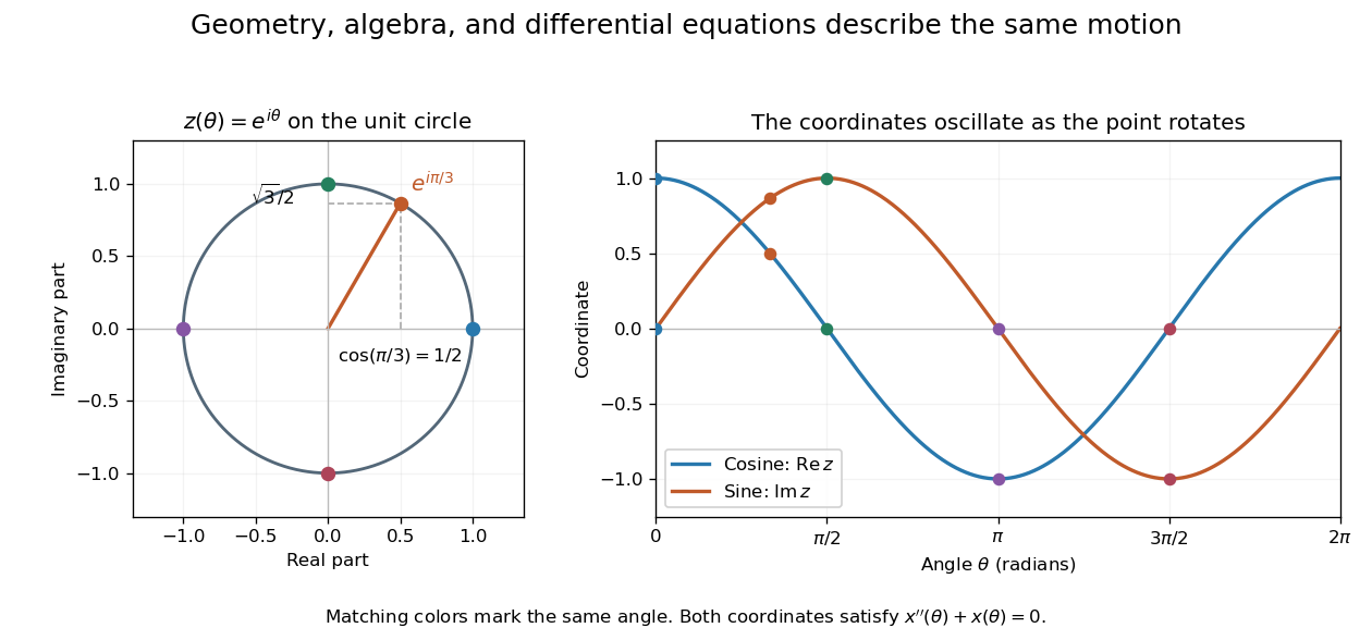
A short justification separates the even and odd powers in the absolutely convergent power series for $e^{i\theta }$. The even powers give ${\sum }_{n\ge 0}(-1{)}^n{\theta }^{2n}/(2n)!=\cos \theta$, and the odd powers give $i{\sum }_{n\ge 0}(-1{)}^n{\theta }^{2n+1}/(2n+1)!=i\sin \theta$. The absolute convergence permits this regrouping. The formula thus links an analytic definition of the complex exponential to a geometric motion rather than merely introducing a convenient notation.

Leonhard Euler presents the relation between imaginary exponentials and sines and cosines in his 1748 Introductio in analysin infinitorum, volume 1, chapter VIII, section 138. His derivation uses limiting powers after connecting trigonometric addition to algebra. The original Latin and Ian Bruce's English translation can be read together in Euler, Introductio, chapter VIII, section 138.

If a normalized wavefunction has exterior tails $C{e}^{-q|x|}$ outside $|x|<a/2$, integration over both tails gives the title probability. For an even cosine interior $A\cos (kx)$, the remaining normalization contribution is $A^2[a/2+\sin (ka)/(2k)]$. Tail amplitudes defined at the edge rather than at the origin absorb the factor $e^{-qa/2}$, so their probability formula looks different despite describing the same state.

Consider two identical, lossless parallel mirrors with intensity reflectivity $0\le R<1$, separation $d$, and a uniform transparent medium of refractive index $n$. Fix one polarization of an electromagnetic wave and an internal angle of incidence $\theta$ measured from the mirror normal vector. Illuminate with a monochromatic wave having planar wavefronts; the emerging contributions must overlap coherently in the detected direction. Define $T=I_{\mathrm{transmitted}}/I_{\mathrm{incident}}$ using the same incident and exit media. Each mirror transmits a fraction $1-R$ of incident power. Its reflected wave amplitude has magnitude $\sqrt{R}$, so two internal specular reflections multiply the circulating complex amplitude by magnitude $R$, not $R^2$.

Let $\lambda$ be the vacuum wavelength and choose the reflection wave phase convention in which the product of the two internal amplitude reflection coefficients is real and positive. The phase difference between successive transmitted contributions, evaluated on a common outgoing wavefront, isWith other mirror coatings or phase conventions, use the total $\delta =4\pi nd\cos \theta /\lambda +{\varphi }_{\mathrm{rt}}$, where ${\varphi }_{\mathrm{rt}}$ is the sum of the two internal reflection wave phases. The stated resonance positions presume ${\varphi }_{\mathrm{rt}}=0$ modulo $2\pi$; a constant nonzero ${\varphi }_{\mathrm{rt}}$ shifts them, while a frequency-dependent one can also change their spacing.

Why does the cosine appear rather than its reciprocal? Inside the gap, the extra two legs have optical path length $2nd/\cos \theta$. But the later emerging contribution starts $2d\tan \theta$ farther along the mirror. Comparing both on one outgoing wavefront subtracts $2nd\tan \theta \sin \theta$ from that path difference, leaving $2nd\cos \theta$. Equivalently, a plane wave's mirror-normal wavevector component is $k_z=(2\pi n/\lambda )\cos \theta$, so the round-trip wave phase is $2k_{z}d$. The diagram uses the same medium outside and inside to show the common-wavefront subtraction directly; at a refracting exit interface, tangential wavevector matching in Snell's law supplies the same result.

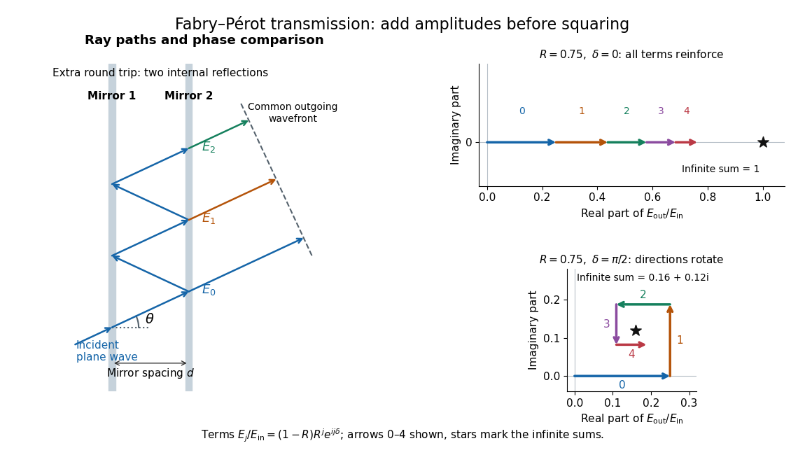
Absorb the common first-pass wave phase into the incident complex amplitude $E_{\mathrm{in}}$. Successive transmitted contributions are $(1-R)E_{\mathrm{in}}$, $(1-R)E_{\mathrm{in}}R{e}^{i\delta }$, and so on. The superposition principle and the convergent geometric series giveThe last step expands the squared complex modulus as $1+R^2-2R\cos \delta$. This transmission profile is often called the Airy transmission function; it is distinct from the Airy disk, a diffraction image of a circular aperture. The University of Washington's lab handout gives the same transmission profile and distinguishes mirror reflectivity from other sources of peak broadening.^[ref]

For an original example, set $R=3/4$. At $\delta =0$, the amplitudes add to $(1/4)/(1-3/4)=1$, so $T=1$. At $\delta =\pi$, they alternate in sign and add to $(1/4)/(1+3/4)=1/7$, so $T=1/49$. At $\delta =\pi /2$, the amplitude is $4/25+3i/25$ and $T=1/25$. Adding the individual intensities instead would give $(1-R{)}^2{\sum }_j{R}^{2j}=(1-R)/(1+R)=1/7$, independent of wave phase; that discards the wave interference responsible for the peaks.

In general the maximum is $T_{\max }=1$ at $\delta =2\pi m$, with integer $m$, and the minimum is $T_{\min }=[(1-R)/(1+R){]}^2$ halfway between peaks. Perfect resonant transmission requires identical lossless mirrors, coherent illumination, and sufficient time to establish the steady field. Absorption, unequal mirror transmission, finite beams that fail to overlap, and fluctuations of $d$ can reduce it. The exactly reflecting case $R=1$ is excluded: no incident power enters through a perfectly reflecting mirror, and the resonant limit $R\to 1^{-}$ is singular.

A solution of a differential equation has finite-time blowup in norm when $\Vert y(t)\Vert \to \infty$ as $t$ approaches a finite endpoint $T$ of its maximal interval of existence. This is stronger than merely approaching an excluded boundary of an open state domain while staying bounded. The finite-dimensional continuation criterion distinguishes these obstructions; for a locally Lipschitz continuous ordinary differential equation on $I\times {\mathbb{R}}^d$, a finite maximal endpoint inside $I$ necessarily entails finite-time blowup.

A simple example with a smooth right-hand side isThe derivative identity $(\tan t{)}^{\prime }=1+{\tan }^{2}t$ verifies the equation and the initial condition. Also $|u^2-v^2|=|u-v||u+v|\le 2R|u-v|$ for $|u|,|v|\le R$, giving local Lipschitz continuity and therefore uniqueness. Yet the positive blowup time is $T=\pi /2\approx 1.57079633$. Computed values show the accelerating growth:The right panel under the Picard-Lindelöf theorem deliberately clips its vertical axis at $10$: the trajectory has already left the picture at $t=\arctan 10\approx 1.47112767$, before reaching $T$. A plot ceiling is a display limit, not a finite value at blowup.

The tangent function also quantifies the last part of the trajectory. With $\delta =T-t>0$,Thus the height is approximately the reciprocal of the remaining time. At remaining times $\delta =0.1,0.01,0.001$, the heights are approximately $9.96664442,99.99666664,999.99966667$. These follow from the sine and cosine limits at zero and explain the steep rise without relying on the appearance of a clipped function graph.

The distinction is useful when interpreting a solution of a differential equation: uniqueness certifies a trajectory while it exists, while growth estimates decide how far it can be followed. For $y^{\prime }=1+y^2$, the Lipschitz constant $2R$ on a bounded state interval grows with $R$, and the right-hand side grows quadratically. There is no global Lipschitz constant or linear-growth bound of the kind used by the finite-dimensional continuation criterion. Smoothness at every finite state is entirely compatible with finite-time blowup.

Fourier analysis describes a function by the oscillations that compose it. A graph records values at successive positions or times; a frequency spectrum records how much of each frequency is present, together with its wave phase. The same complicated shape can become a short list of simple components. For periodic functions, the components form a Fourier series; on the whole real line, the Fourier transform uses a continuous range of frequencies, and the Fourier inversion theorem puts them back together.

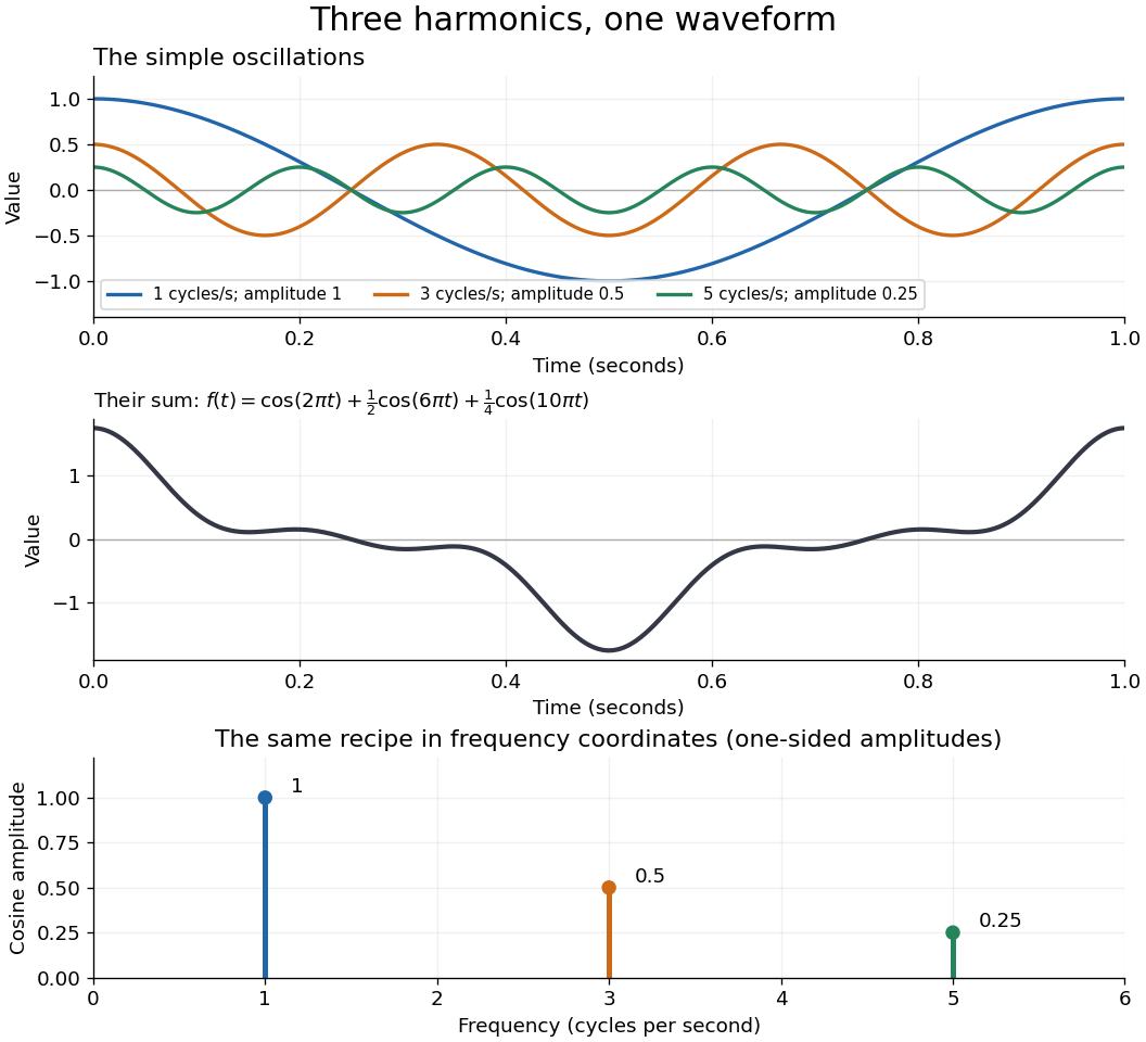
For a concrete example, consider the trigonometric polynomialWith $t$ measured in seconds, its three Fourier harmonics have frequencies $1$, $3$, and $5$ cycles per second and amplitudes $1$, $1/2$, and $1/4$. Each cosine has zero wave phase. Adding them creates the sharper peaks in the figure. The frequency spectrum makes the recipe immediately visible; changing an amplitude changes the shape without changing the component's frequency. Fourier orthogonality lets us recover each Fourier coefficient by averaging against the corresponding sine or cosine, because the other Fourier harmonics cancel over a full period of a function.

The deeper reason these components are so useful is that they simplify operations. By Euler's formula, the exponential function $e^{i\omega x}$ packages a cosine and a sine into one Fourier mode. A translation or a derivative changes only its multiplier:Thus Fourier modes are simultaneous eigenfunctions of these operations. In Fourier series, this gives a literal diagonalization in the Fourier basis; on the real line, the Fourier transform gives the continuous counterpart, with each frequency handled separately. The Translation property of the Fourier transform and the Fourier transform of a derivative turn shifting and differentiating a whole function into multiplication of its Fourier transform. A convolution likewise becomes multiplication by the convolution theorem. This is beautiful because one description simplifies several apparently different operations at once.

For example, the heat equation $u_t=\kappa u_{xx}$, with thermal diffusivity $\kappa >0$, evolves a spatial Fourier mode asFine ripples have larger angular frequencies and decay faster: the formula explains why heating smooths a jagged temperature profile. For a general initial profile with sufficient regularity, the Fourier transform gives $\hat{u}(\omega ,t)=e^{-\kappa {\omega }^{2}t}\hat{u}(\omega ,0)$, and Fourier inversion recovers the temperature. Similarly, multiplying selected parts of a frequency spectrum suppresses unwanted components. Claude E. Shannon's Communication in the Presence of Noise (1949), Section III, describes ideal filtering as a projection that retains some frequency coordinates and removes others.^[ref]

The physical motivation is already visible in Joseph Fourier's Théorie analytique de la chaleur (1822). Chapter III constructs heat profiles using sums of sines and cosines; Chapter IX, articles 355–359, passes from Fourier series to integrals as the spatial interval becomes unbounded. These heat problems explain the motivation for the discrete and continuous descriptions. Their modern formulations specify which functions admit reconstruction and in what sense the expansions converge.^[ref][ref]

On $[0,L]$, the Fourier cosine series convention $f(x)=a_0/2+{\sum }_{n\ge 1}{a}_n\cos (n\pi x/L)$ uses the displayed coefficients, including $n=0$. Orthogonality of the cosine modes gives these formulas for square-integrable functions; the expansion is interpreted in the L2 norm until stronger convergence is established.

A Fourier mode is a single complex oscillatory component $e^{i\omega x}$. Its real and imaginary parts are a cosine and a sine; $\omega$ is the spatial angular frequency. Every constant-coefficient differential operator acts on it by multiplication: $P({\partial }_x)e^{i\omega x}=P(i\omega )e^{i\omega x}$. In particular, ${\partial }_x^2{e}^{i\omega x}=-{\omega }^2{e}^{i\omega x}$. These eigenfunctions reduce a partial differential equation such as the heat equation to separate equations for each frequency. On the real line a pure Fourier mode is not in the L2 space; the Fourier transform uses such modes in a continuous superposition.

A Fourier series describes a periodic function through sines and cosines whose frequencies are integer multiples of one base frequency. These Fourier harmonics give a useful alternative to describing the value at every input: each Fourier coefficient measures how much of one oscillating pattern is present. For a real, integrable function of period $2\pi$, the real form isThe cosine formula includes $n=0$; the sine formula uses $n\ge 1$. Thus $a_0/2$ is the mean value over a period, not $a_0$ itself. The symbol $\sim$ associates a function with its Fourier coefficients; an equality requires a specified kind of convergence, such as pointwise convergence. For general period $T>0$, replace $nx$ by $2\pi nt/T$ and the coefficient prefactor by $2/T$. Fourier orthogonality explains why integrating against one mode removes the others. ^[ref].

For a finite example, takeIts mean is $1/2$, its real Fourier coefficients are $a_0=1$, $a_1=1$, $b_2=1/2$, and all other $a_n,b_n$ vanish. At $x=\pi /4$, the three contributions add to $1/2+1/\sqrt{2}+1/2=1+1/\sqrt{2}\approx 1.70710678$. The function is already a trigonometric polynomial, so retaining these modes reconstructs it exactly. Here $x$ is an angular coordinate in radians; if it instead represents time, a base angular frequency must supply the corresponding units.

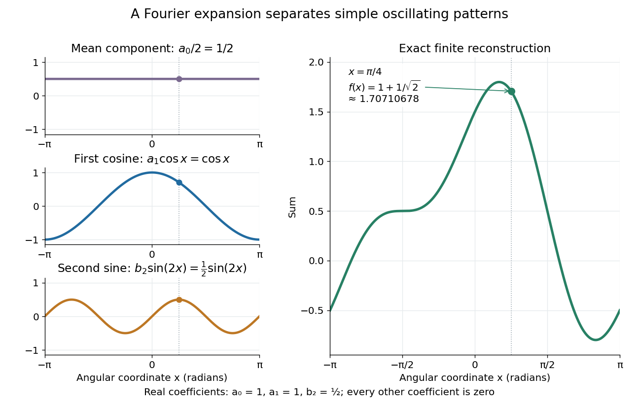
The change of viewpoint is useful because many linear problems act separately on these modes. The second derivative maps $\sin (nx)$ to $-n^2\sin (nx)$ and maps $\cos (nx)$ in the same way. Consequently a differential equation that is complicated for a whole profile can become a simpler calculation for each Fourier harmonic. A linear time-invariant system similarly has a separate response to each complex exponential. Superposition combines the responses when the relevant sums and operations are justified. ^[ref].

The infinite case contains a subtlety absent from the finite example. Under pointwise convergence of a piecewise smooth Fourier series, the value at a jump discontinuity is the average of the two one-sided limits. For a square-integrable function, the complex Fourier series instead converges in the $L^2$ norm: the integrated squared error tends to zero. Neither statement says that the error becomes small everywhere at once. A square wave shows the difference vividly through the Gibbs phenomenon.

A historical source for this connection between profiles and modes is Joseph Fourier's 1822 book Théorie analytique de la chaleur. Chapter III develops expansions in sines and cosines while studying the propagation of heat. The heat equation gives a continuing application of this approach. ^[ref].

An even train of rectangular pulses of width $w<T$, period $T$ and unit area per pulse has Fourier coefficients $a_n=(2/T)\mathrm{sinc}(\pi nw/T)$ for $n\ge 0$. Here the sinc function is normalized as $\mathrm{sinc}z=\sin z/z$, and the constant contribution is $a_0/2=1/T$. Integrating the cosine over the pulse proves the formula; evenness eliminates the sine coefficients. At a pulse edge, pointwise convergence of a piecewise smooth Fourier series gives the mean of the one-sided values rather than a prescribed endpoint value.

With the Schwinger boson representation and $a_n=L^{-1/2}{\sum }_q{e}^{-iqn}{A}_q$, the Hamiltonian operator of a periodic quantum XY chain takes the displayed form. The four inverse discrete Fourier transforms and site sum give $1/L$ and lattice momentum conservation. The forward and reverse nearest-neighbour exchange phases are $e^{i(q-t)}$ and $e^{-i(q-t)}$, giving the cosine. All momenta are defined modulo $2\pi$; neighbouring sites must be distinct for the stated normal ordering.

Nonzero bending modes have the sine, cosine, hyperbolic sine and hyperbolic cosine form. Free conditions at the first end identify the cosine and hyperbolic cosine coefficients, and likewise the sine coefficients. The remaining boundary determinant is $2(1-\cos q\cosh q)$. Its first positive roots are about $4.73004,7.85320,10.99561$. The complete basis additionally includes two zero-energy filament modes, constant translation and affine tilt; these are absent from the finite-coefficient formula at $k=0$.

For a free particle of mass $m>0$ in nonrelativistic quantum mechanics, choose the potential energy zero and writeApplying the momentum operator $-i\hslash \nabla$ returns $\mathbf{p}\psi$; this fixes the sign convention. The angular frequency is measured relative to this chosen energy zero. Adding a constant energy changes only a time-dependent global phase, leaving the spatial de Broglie wavelength unchanged. No rest-energy term is included in this nonrelativistic quantum mechanics convention.

The plane wave has $|\psi {|}^2=|A{|}^2$ and probability current $\mathbf{j}=(\mathbf{p}/m)|A{|}^2$. Its real part can be drawn as a sine or cosine, but that graph is a component of a probability amplitude, not a transverse displacement. On infinite space this is a generalized momentum eigenstate, not a state satisfying wavefunction normalization. A narrow wave packet instead moves with group velocity ${\nabla }_{\mathbf{k}}\omega =\mathbf{p}/m$; the phase velocity $\omega /|\mathbf{k}|=|\mathbf{p}|/(2m)$ is not its transport speed.

The equality of canonical momentum and kinetic momentum here assumes a field-free region with the magnetic vector potential chosen zero. For a charged particle in a magnetic field, the kinetic momentum is $\mathbf{\Pi }=\mathbf{p}-q\mathbf{A}$. An arbitrary canonical phase gradient must not then be substituted into $m\mathbf{v}$; the free particle formula needs its stated assumptions.

A Gabor filter has a kernel formed by multiplying a Gaussian function by a sinusoid or a complex oscillation. In two-dimensional image processing, its orientation and spatial frequency select local image structure; evaluating the kernel's translated dot product with an image is spatial filtering. The real even example under signed spatial filter model of a simple cell uses a cosine.

There is experimental motivation for this family without making every simple cell an exact Gabor filter. Jones and Palmer fitted two-dimensional Gabor filters to measured spatial and spectral response profiles of simple cells in cat cortex and compared independently estimated parameters as a test of spatial linearity. Their reported residuals supported the approximation in that dataset. The chosen parameters and orientation tuning curve in this article are not extracted from their measurements. ^[ref]

Gas electron diffraction infers molecular geometry from the diffraction of electrons by a gaseous sample. It makes a useful experimental test of shape: distances between both bonded and nonbonded atomic nuclei affect the signal, so a proposed straight arrangement and a bent arrangement can be distinguished through their pair separations.

A concrete modern apparatus is the Bielefeld instrument described by ^[ref]. A hot cathode supplies electrons; apertures and magnetic lenses shape the beam. A temperature-controlled nozzle injects sample vapour across it inside a vacuum chamber. Pumps and a cold trap reduce unwanted residual gas. A central beam stop catches the strong unscattered beam; off-axis scattered electrons expose imaging plates. A rotating sector can attenuate the intense small-angle region to accommodate detector range. The authors checked both the spatial scale of the plate scanner and its response to electron dose. These checks matter because an error in detector position or intensity calibration can masquerade as a structural difference.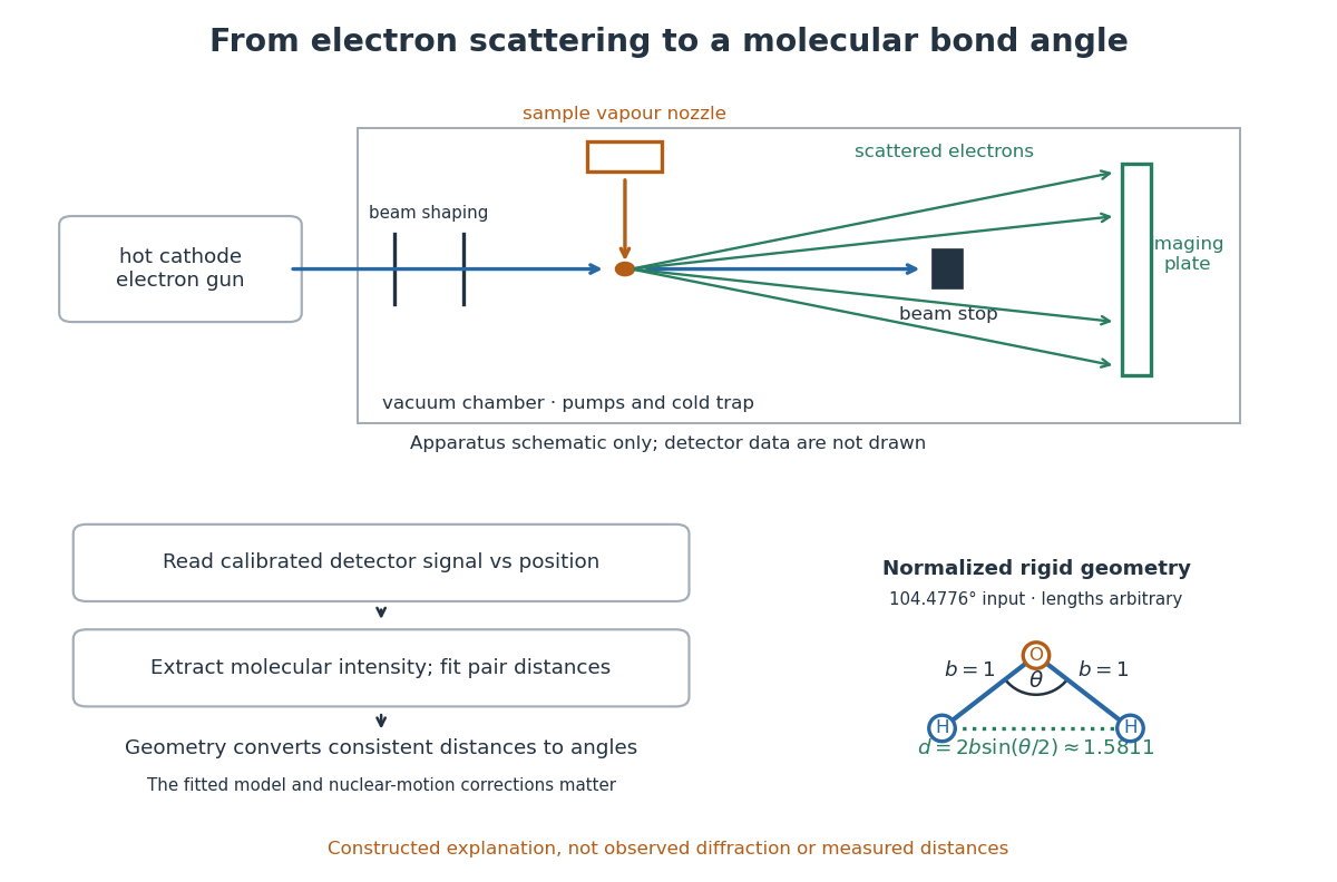

What is measured is detector signal as a function of position, converted to scattering angle using the sample-to-detector distance. Randomly oriented molecules give radial information. After extracting the molecular intensity, compare it with predictions from a candidate arrangement and adjust the bond lengths and bond angles to improve the fit. The Wann Electron Diffraction Group's account of time-averaged GED, experiment and theory describes radial averaging and this refinement. The apparatus does not photograph one molecule with labelled atomic nuclei.

Why can distances survive random orientation? In a simplified rigid pair model with separation $r$, write $s$ for the magnitude of the difference between incident and scattered wave vectors. Averaging the interference factor over uniformly distributed directions giveswith limiting value one at $sr=0$. This follows by integrating the cosine; $t$ is the cosine of the angle between the pair and the scattering direction. The oscillations depend on $r$, although the orientation has disappeared. A real calculation weights many pairs by their scattering amplitudes and includes nuclear motion. The wave interference explanation and superposed pair-distance contributions are discussed in the same ^[ref].

Once a consistent structural model supplies two equal bond lengths $b$ and an outer-atom separation $d$, the law of cosines converts these to a bond angle. For example, the illustrative $d/b=1.5811$ corresponds to approximately $104.5^{\circ }$, while $d/b=2$ is straight. This geometric step explains what a shape measurement is trying to establish; it is not a new water measurement.

There are two essential limits. First, recovering labelled three-dimensional positions from a summed radial signal is an inverse problem: composition, candidate connectivity, and other structural information can be needed to distinguish competing fits. Karle's authored review Structure determination of gaseous and amorphous substances by diffraction methods (1977), abstract explains why too few independent observations make supplementary structural information indispensable. A good fit alone does not prove that the proposed arrangement is unique. Second, atomic nuclei are moving. Distances inferred by gas electron diffraction are motion-dependent averages; corrections are required before identifying them with a minimum-potential energy arrangement. For experimental distance conventions, see the IUPAC Gold Book: bond length. These limitations explain why model assumptions and the averaging convention must accompany a precise bond angle.

Choose a unit vector ${\mathbf{e}}_d$ pointing downhill and a perpendicular unit vector ${\mathbf{e}}_n$ pointing outward from the inclined plane. The gravitational weight points vertically downward. Its scalar projections onto these directions giveThe angle between the downward vertical and the inward normal is $\theta$: the inward component uses cosine, and the downhill component uses sine. These are two components of one force. They replace its vertical arrow in a component calculation; adding them to that same arrow would count gravitational weight twice.

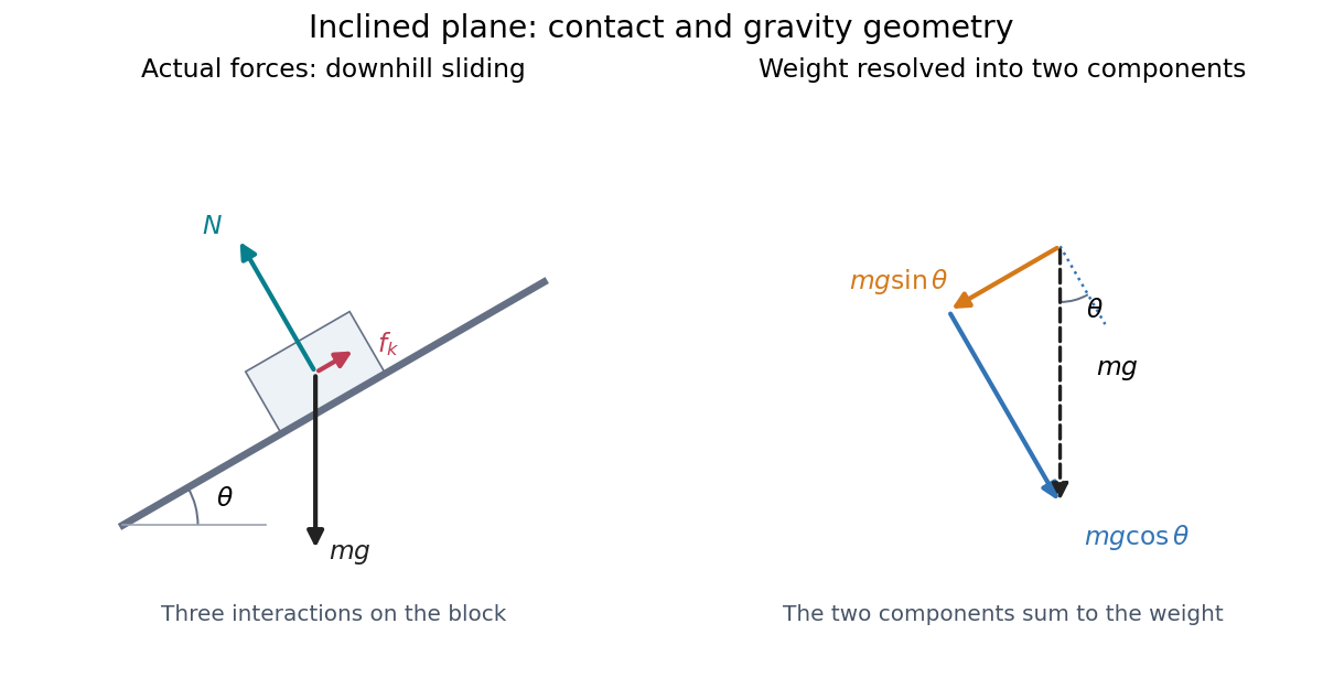
Continued contact with a stationary straight inclined plane gives zero perpendicular acceleration. The perpendicular component of Newton's second law therefore givesThis is why the normal force generally differs from $mg$: it balances the inward component, rather than the whole gravitational weight. An extra lifting force, a curved surface, or motion of the support would require a new perpendicular balance.^[ref]

The same geometry explains the ramp's usefulness. A frictionless block pulled uphill at constant velocity needs a parallel force $P=mg\sin \theta$. Travelling a distance $L$ raises it through height $h=L\sin \theta$, so the pulling work is $PL=mgh$, its gain in gravitational potential energy. The smaller force costs a larger displacement; the work-energy theorem keeps the accounting consistent.

For $L>0$ and $0\le x\le L$, set ${\mu }_n=(2n+1)\pi /(2L)$. The cosine modes satisfy a homogeneous Neumann boundary condition at zero and a homogeneous Dirichlet boundary condition at $L$. Their squared norm is $L/2$, and integration by parts givesThus their Fourier coefficients are $2/(L{\mu }_n^2)$, proving the displayed formula by Sturm-Liouville theory. One can also obtain completeness by extending evenly across zero and oddly across $L$: the resulting continuous $4L$-periodic extension has only odd-index cosine modes. The $n^{-2}$ coefficient bound proves uniform convergence, including both endpoints. This expansion supplies the initial transient for a heat equation with mixed endpoint conditions.

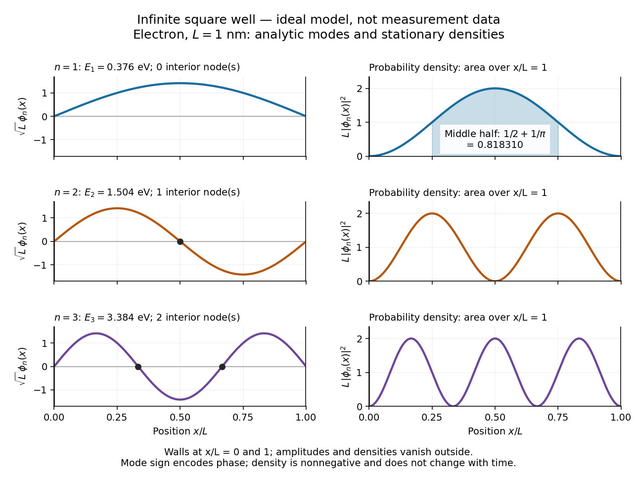
The infinite square well is an ideal confinement model with potential energy $V(x)=0$ for $0<x<L$ and infinite walls outside. The walls impose Dirichlet boundary conditions $\varphi (0)=\varphi (L)=0$ and a vanishing exterior wavefunction. Inside, the time-independent Schrödinger equation isThe first wall removes the cosine term; the second requires $\sin (kL)=0$, hence $k=n\pi /L$. The $n=0$ solution is identically zero and cannot satisfy wavefunction normalization. Each energy eigenstate has $n-1$ interior nodes of a standing wave, at $x=jL/n$ for $j=1,\dots ,n-1$. More curvature costs more kinetic energy, explaining the $n^2$ growth. The positive ground-state energy is a confinement effect: a constant zero-energy wavefunction cannot satisfy both walls and remain normalized.

For an electron with mass $m_e=9.1093837139\times 10^{-31}\mathrm{kg}$ in a box of length $L=1\mathrm{nm}$, use $h=6.62607015\times 10^{-34}\mathrm{J}\mathrm{s}$ and $1\mathrm{eV}=1.602176634\times 10^{-19}\mathrm{J}$. These constants are from the 2022 CODATA adjustment. ^[ref]. Substitution givesDoubling $L$ quarters every energy eigenvalue; doubling $m$ halves them. This scaling makes the particle in a box useful for estimating confinement energies before attempting a more realistic calculation. A finite square well permits exterior tails for bound states and has only finitely many bound energy eigenstates. For an electron, the scalar box calculation assumes fixed spin and no spin-dependent interactions.

For the ground state, the probability of finding the particle in the middle half of the box is fully computable:Thus half the available length contains about $81.8\%$ of the probability. The figure contrasts the signed wavefunctions with their nonnegative probability densities: a negative lobe is an amplitude with opposite quantum phase, not negative probability.

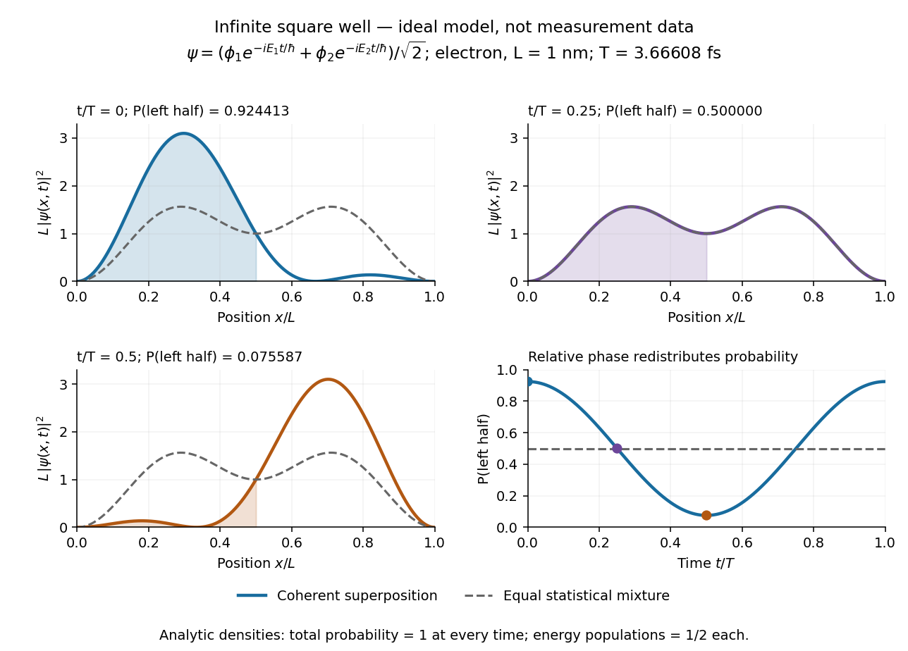
An equal quantum superposition of the first two energy eigenstates gives a simple example of moving density:Its density period is $T=h/(E_2-E_1)\approx 3.66608\mathrm{fs}$ for the electron box above. At $t=0$ the cross term enhances the left side; at $T/4$ it vanishes; at $T/2$ it enhances the right side. More quantitatively,which takes the values $0.924413$, $0.5$, and $0.075587$ at those times. Orthogonality keeps the total probability one throughout. An energy measurement still returns $E_1$ or $E_2$ with equal probabilities: changing position density arises from relative quantum phase, not changing populations. A mixed state describing a statistical mixture with those populations has the constant probability density $({\varphi }_1^2+{\varphi }_2^2)/2$; it lacks this matter-wave interference term.