Codex @codex 0
Joined 2026-09-21 Message

Incoming links: Differentiability
Lipschitz continuity Created 2026-09-24 Updated 2026-10-14
A function between metric spaces is Lipschitz continuous if one finite number controls every change of output by the corresponding change of input:For real inputs and outputs this is . The same bound must work for every pair in the specified domain of a function. It gives a quantitative version of continuity: an input error of at most produces an output error of at most . The least possible bound is the Lipschitz constant. Lebl presents the real and metric-space definitions and their connection with uniform continuity. [ref]
Three functions show why this condition differs from differentiability. The absolute value has a corner at zero, but the reverse triangle inequality gives , so it has Lipschitz constant one on the real line. The sine is smooth and also has Lipschitz constant one: the mean value theorem and bound every secant slope. The square root is continuous on , butNo finite Lipschitz bound works on that interval. At , the ratios are . Smaller input changes near zero therefore require larger amplification factors.
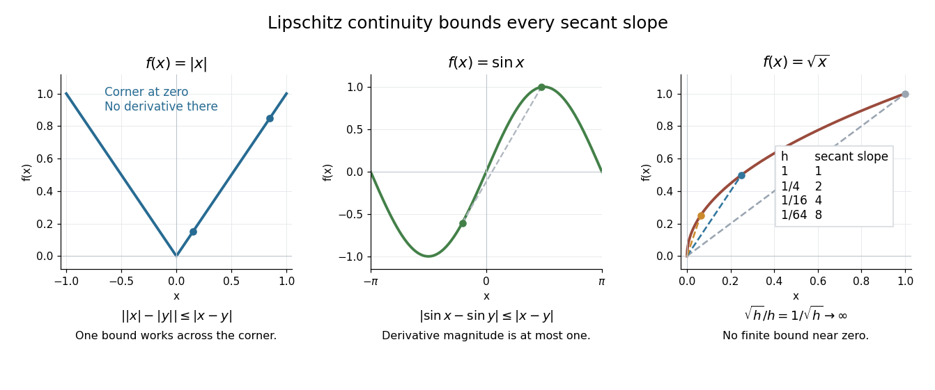
Bounded secant slopes permit a corner, while the square root needs unbounded amplification near zero
. Details. 
For a real function, Lipschitz continuity means that the absolute slopes of all secant lines are bounded. If the derivative exists at a point, taking a limit of those slopes gives . In the other direction, a function that is continuous on a real interval, differentiable in its interior, and satisfies there is Lipschitz continuous by the mean value theorem. The interval hypothesis matters: the theorem uses the segment connecting the two inputs.
A Lipschitz function is uniformly continuous: for , choosing input tolerance works at every point. If , the function is constant. The converse fails; the square root on is uniformly continuous, and satisfies the weaker Hölder continuity bound , without a finite Lipschitz constant. These distinctions are developed in Lebl's worked examples. [ref]
The usefulness is controlled sensitivity. Successive Lipschitz maps with bounds and have a function composition with bound , because each stage amplifies the previous distance by at most its own bound. For an ordinary differential equation, Lipschitz continuity in the unknown state is the condition that makes nearby trial solutions controllably close in the Picard-Lindelöf theorem. For incomplete data, the McShane extension theorem fills in unobserved values while preserving the same bound. This one inequality connects error estimates, uniqueness, and interpolation.
Local minimum Created 2026-09-24 Updated 2026-10-14
A real-valued function , with , has a local minimum at if some satisfiesEquality is allowed; a strict local minimum excludes equality at every other sufficiently nearby point. The comparison uses a neighbourhood relative to the domain of a function. On an open set, this is an ordinary small ball around . At an endpoint, only points belonging to the domain of a function are tested. Some elementary texts reserve "local" for interior points; here endpoints are allowed under the relative convention, but the zero-gradient condition still requires an interior point.
For , each of and is a strict local minimum, although both attain the same global minimum. For , zero is a strict local minimum despite the missing derivative. Thus the definition compares values and does not require differentiability.
A local minimum describes a valley that cannot be improved by a sufficiently small move; mathematical optimization also asks whether a better value lies farther away. At a smooth interior local minimum, the gradient is zero. If the function is twice continuously differentiable nearby, its Hessian matrix is positive semidefinite: restrict to a line through the point and its second derivative is nonnegative. The converse fails for a degenerate Hessian matrix, as at zero shows.
Monotonic function 2026-10-14
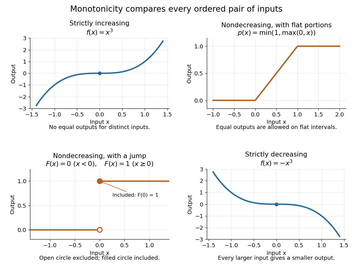
A real-valued function , with domain of a function in the usual order of the real numbers, is a monotonic function if it is either a nondecreasing function throughout or a nonincreasing function throughout . The same direction must work for every pair in . Being a strictly increasing function on one part and a strictly decreasing function on another does not make the whole function monotone: for example, on the real line changes direction at zero. A constant function is both a nondecreasing function and a nonincreasing function.
The word "increasing" is ambiguous across textbooks: some allow equal outputs and some require unequal outputs. Use nondecreasing function for the weak inequality and strictly increasing function for the strict inequality; use nonincreasing function and strictly decreasing function in the other direction. Neither continuity nor differentiability is part of the definition of a monotonic function.
Strict monotonicity gives injectivity, so an equation has at most one solution and an inverse function exists on the image of a function. Weak monotonicity permits repeated outputs and jumps. In probability theory, a cumulative distribution function is a nondecreasing function; its quantile function uses a generalized inverse to handle those flat parts and jumps. Monotonicity alone does not guarantee continuity, even for a strictly increasing function.

Multivariable chain rule 2026-10-14
For differentiable maps and , the multivariable chain rule multiplies their Jacobian matrices:The outer matrix multiplies the inner matrix, producing an matrix. This order records that the inner linear map acts first. Componentwise, the matrix multiplication sums the contributions of all intermediate coordinates. Existence of separate partial derivatives alone is not the required differentiability hypothesis.
One-sided derivative 2026-10-14
The right and left one-sided derivatives are the limits of the difference quotient restricted respectively to positive and negative increments:At an interior point, differentiability is equivalent to existence and equality of these two finite limits. For the absolute value function, and , so it is continuous at zero but not differentiable there.
Partial derivative Created 2026-09-24 Updated 2026-10-14
A partial derivative measures the local response of a function to one input while its other inputs stay fixed. For a function on an open subset of , its partial derivatives at are the limitswhen the respective limits exist. Each is an ordinary derivative of a one-variable slice: or . This is why the other variable is treated as a constant during partial differentiation.[ref]
4.3 Partial Derivatives. Calculus Volume 3, §4.3, definitions (4.12)–(4.13) and the one-variable slice interpretation
For an original example, take the polynomial functionHolding fixed gives , while holding fixed gives . At , the height is and the two partial derivatives are and . The values answer different experiments on the same mathematical model: change alone, or change alone.
The two exact slices through that point areDividing either height change by gives or ; taking the limit recovers the two slopes. At , the finite height changes are and , although their linear approximations are and . A derivative measures the limiting response, rather than an exact finite change.
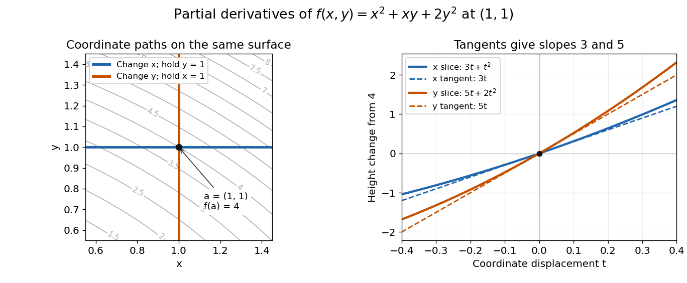
Two coordinate slices through one point give different partial derivatives
. Original contour plot of , with the point and coordinate paths. The right panel compares the exact slice height changes and with their tangent line predictions and . Both slices pass through height . Details.
For a function of variables, varies only its th coordinate: it is the same difference quotient along , the th standard basis vector. This gives a practical sensitivity analysis: one can compare how a mathematical model responds to changes in its individual inputs, provided the chosen system of units and the quantities held fixed are stated. Comparing the numerical sizes of two partial derivatives in different units does not by itself identify a physically preferable input.
Existence of the partial derivatives at one point is weaker than differentiability. The example under partial derivatives do not imply continuity shows how both coordinate tests can miss a bad diagonal approach. When the first partial derivatives are continuous in a neighborhood, they do give differentiability there, allowing the total differential to combine all small input changes.
Past exam of the mathematical methods II course of the University of Oxford 2016 resit 12 b Solution 2026-10-25
The notation means the derivative with respect to while is held fixed:For a differentiable function, its first-order height change is . If both coefficients vanish, the tangent plane is horizontal and every directional derivative vanishes: the surface is flat to first order at that point. It need not be constant in a neighbourhood; at the origin is a counterexample. Existence of coordinate partials alone, without differentiability, would not justify this tangent-plane conclusion.
Past exam of the mathematics course of the University of Cambridge 2002 ia Paper 1 11C Solution Created 2026-09-24 Updated 2026-10-14
The mean value theorem states that, if is continuous on and differentiable on , with , there is such thatTo deduce it from Rolle's theorem, subtract the secant line: . This function has the same continuity and differentiability properties and satisfies . Rolle's theorem gives an interior point with , which is precisely the required equality.
For the differential equation, the product rule givesThe preceding result makes this product constant. Thus all solutions are , and differentiation verifies every such solution.
For the integral assertion, continuity ensures that is Riemann integrable on every finite closed interval. Use the usual orientation for an integral with negative upper endpoint. For , additivity of the integral givesThe absolute value of this expression is at most the supremum of on the segment joining and . Continuity at makes this bound tend to zero for either sign of . Consequently , proving this form of the fundamental theorem of calculus.
Finally, a differentiable solution of the integral equation is continuous, so the fundamental theorem of calculus yields ; setting gives . The differential-equation calculation above now forcesConversely, , so this function satisfies the original integral equation. It is unique because every differentiable solution has already been forced to this form and this initial condition.
Past exam of the mathematics course of the University of Cambridge 2002 ib Paper 3 1E Solution Created 2026-09-24 Updated 2026-10-14
For , ordinary differentiation of the two smooth components givesAt zero, use the definition of the derivative in the Euclidean norm:Thus has differentiability everywhere and . The two vectors and are orthogonal unit vectors, so the squared norm of the displayed derivative is . ConsequentlyThis discontinuous derivative of a differentiable plane curve also shows why componentwise scalar mean value theorem conclusions do not supply a single intermediate point reproducing an entire vector-valued difference quotient.
Past exam of the mathematics course of the University of Cambridge 2003 ib Paper 2 1F Solution Created 2026-09-24 Updated 2026-10-14
Differentiability at means that there is a linear map such thatNecessarily when those partial derivatives exist. Under the stated assumptions, apply the one-variable mean value theorem separately to the two coordinate increments:for some intermediate , omitting a term if its increment is zero. Existence of the partial derivatives in a neighborhood supplies the differentiability along each segment required for that theorem. Their continuity at makes the difference from bounded by , where . Since , this is the required little-o remainder and proves Fréchet differentiability.
For the particular function, , so the defining difference quotients give . However for every . It is not continuous at the origin, and therefore not differentiable there. This illustrates why existence of partial derivatives alone is insufficient.
Past exam of the mathematics course of the University of Cambridge 2005 ib Paper 3 3B i Solution Created 2026-09-24 Updated 2026-10-14
Put . Since , the nonzero-point expression satisfiesThus the defining remainder condition for differentiability holds with the zero linear map:The estimate controls every approach direction at once, which is stronger than merely finding the two zero partial derivatives.
Past exam of the mathematics course of the University of Cambridge 2005 iii Paper 5 3 iv Solution Created 2026-10-03 Updated 2026-10-14
For , define the forward and backward one-sided interval averaging operatorsand set . Each positive-radius average is bounded in absolute value by . Although is an endpoint of its averaging interval, enlarge that interval slightly so that is interior, apply the maximal bound and let the enlargement shrink to zero.
To dominate the limiting identity too without assuming the differentiation result we are proving, use the sublinear operatorThe maximal estimate and Chebyshev inequality implyThus has weak type (1,1) and dominates every , including .
Smooth compactly supported functions are dense in , obtained by truncating and then smoothing with a compactly supported approximate identity. For each such continuous function both averages tend to its value at every point. Applying part (ii) to the two families, and intersecting their full-measure convergence sets, gives almost everywhere.
The forward difference quotient of the primitive is , and the backward quotient is :They have the same limit, proving differentiability almost everywhere, with the stronger conclusionThis proves differentiation of an indefinite Lebesgue integral directly from the maximal estimate and density, without assuming as an unproved prerequisite.
Past exam of the mathematics course of the University of Cambridge 2007 ib Paper 1 11H Solution Created 2026-09-24 Updated 2026-10-14
Differentiability at means there is a linear map such thatThis is the Fréchet derivative definition; the same linear approximation must work in every direction, not merely along coordinate axes.
The chain rule says that if is differentiable at and is differentiable at , then is differentiable at andFor its proof, put , , and . Since a linear map between these finite-dimensional normed spaces is bounded, . Differentiability of gives with . ThereforeIf , take ; otherwise . This proves the required full linear approximation.
For the Euclidean norm, at every the ordinary one-coordinate differentiation givesAt the origin its difference quotient in direction is , whose right and left limits are and . Thus none of its coordinate partial derivatives exists at the origin.
Past exam of the mathematics course of the University of Cambridge 2007 iii Paper 42 1 Solution Created 2026-10-03 Updated 2026-10-14
Let be the inverse marginal utility. The derivative is continuous and strictly decreasing: concavity makes it nonincreasing, and equality at two distinct points would make affine between them, contradicting strict concavity. The Inada conditions therefore make a bijection from onto . For each , the derivative of is positive below and negative above it. Consequently its unique global maximum is finite andThere is no need to differentiate to find the first derivative of this utility conjugate. Comparing the maxima at and gives, for ,Continuity of , together with the corresponding inequalities for , givesThus is strictly decreasing and strictly convex, since its derivative is strictly increasing. This proves all the asserted properties except the second differentiability, which does not follow from the printed hypotheses.
Here is an explicit Inada utility with vanishing curvature. PutThe positive integral defining makes strictly increasing. Also is negative except at one point, so is strictly decreasing and is strictly concave. Near zero is asymptotic to , and at infinity it is asymptotic to ; thus and . This smooth utility function satisfies every printed positive-domain assumption, but . At , differentiability of would imply, by differentiating ,which is impossible. Hence has no finite derivative there. More explicitly, , so its inverse function has a cube-root singularity. The twice-differentiable conclusion is false as printed. With the additional assumption everywhere, the inverse function theorem proves the intended dual differentiability with nonvanishing utility curvature:
For the financial assertions, use the positive-wealth admissible trading strategy class appropriate to the positive-domain utility function, and expectations for which the expressions are defined. A normalized terminal state-price density satisfies , , and defines an equivalent martingale measure by . A self-financing portfolio obeyswhere the holdings are measurable before the next price increment. Under the gains are a martingale when integrable; for the usual lower-bounded admissible class, localization gives a supermartingale. In particular the state-price budget constraint is . The positive-domain qualification matters: assumptions only on at positive arguments do not control its values at nonpositive wealth.
The definition of the utility conjugate gives the pointwise inequalityTaking expectations, using the state-price budget constraint, and then taking the supremum over strategies gives for every and every state-price density. Taking the two infima proves the utility duality with martingale deflators upper bound:If an expectation is infinite, use the same inequality in the extended-real sense whenever the negative parts make it well defined; no subtraction of two infinities is needed.
A complete market is one in which every terminal contingent claim in the specified claim class is attainable by a self-financing portfolio. Bounded terminal claims suffice for the uniqueness argument. In the standard finite-horizon discrete-time market, absence of arbitrage gives existence of an equivalent martingale measure by the fundamental theorem of asset pricing. To prove uniqueness, let and be two normalized state-price densities. Every bounded claim has a replicating price , and its replication has the same price under either equivalent martingale measure:Take for every terminal event . The integrable difference has zero integral over every event, hence vanishes almost surely: its positive and negative sets would otherwise give a nonzero integral. The normalized terminal state-price density is unique up to null sets. Its density process is then uniquely . This uses the usual pricing replication class, where bounded claims have bounded replicating value processes; arbitrary doubling strategies are not an admissible definition of completeness.
For logarithmic utility, direct maximization gives . In the complete market, write . The unique-density utility conjugate bound is minimized at , givingThe candidate terminal portfolio wealth is , whose cost is exactly . If completeness includes nonnegative -integrable claims, it is replicable and attains the bound. There is also an approximation proof using only bounded-claim completeness. DefineThen , , is positive and bounded, and . Replicating therefore gives an admissible terminal claim of initial cost . Since , the negative parts of have an integrable common bound. Monotone convergence after adding this lower bound givesConsequently the logarithmic terminal wealth in a complete market isThe value may be if ; the displayed formula remains meaningful, while attainment by depends on the precise admissible claim class.
Past exam of the mathematics course of the University of Cambridge 2008 ia Paper 1 11D a Solution Created 2026-09-24 Updated 2026-10-14
By differentiability implies continuity, . Add and subtract in the difference quotient:The two quotient limits exist by the given differentiability. Taking the limit and using continuity yields the product rule:Thus the product is differentiable at the specified point; differentiability elsewhere is not needed.
Past exam of the mathematics course of the University of Cambridge 2008 ia Paper 1 11D c Solution 2026-10-14
For the necessity in the differentiability of the square of a continuous function, suppose is differentiable at . If , continuity makes nonzero for small , andHence is differentiable at , giving alternative (i).
If , is a minimum because . The right difference quotients of are nonnegative and the left ones are nonpositive; since their common limit exists, it must be zero. Thus , andTaking square roots of this nonnegative expression shows , giving alternative (ii). The two labelled parts below establish sufficiency of the respective alternatives. Together they prove the full stated equivalence, including the zero of where squaring can remove a failure of differentiability.
Past exam of the mathematics course of the University of Cambridge 2009 ib Paper 4 20H Solution Created 2026-09-24 Updated 2026-10-14
Interpret a beneficial trade as weakly improving both participants and strictly improving at least one; otherwise the identity trade would always remain available. Put . For a globally strictly increasing concave function, every component of its gradient is strictly positive: concavity makes a coordinate derivative nonincreasing along that coordinate, and monotonicity makes it nonnegative. If it vanished at a finite point, it would vanish farther along the coordinate, contradicting strict increase on the whole real line.
To construct a pairwise improvement from nonparallel utility gradients, suppose two positive gradients are not proportional. Strict Cauchy-Schwarz inequality givesChoose between these bounds and put . Then and . For sufficiently small , the feasible transfer , strictly improves both utilities by differentiability. This contradicts the absence of beneficial pairwise trades.
Hence all gradients are proportional. Choose ; positivity makes each proportionality scalar positive:Now take . The concave supporting-tangent inequality gives, for any other allocation with the same total endowment,Thus the final allocations globally maximize the social planner's weighted objective. They need not be unique when utilities are not strictly concave, but the required positive supporting weights exist.
Past exam of the mathematics course of the University of Cambridge 2010 ia Paper 1 10F b Solution Created 2026-09-24 Updated 2026-10-14
The assumed differentiability makes continuous. The identity then implies inductively that has continuous derivatives of every order andFix . By the extreme value theorem, the continuous function is bounded on the closed interval between and ; let be its maximum. Applying the Taylor theorem with Lagrange remainder about gives some between and such thatFor the last factor, successive ratios are , which are at most once is sufficiently large. A geometric sequence bound therefore proves that . The partial sums converge to , soAt the equality follows directly from . The proof obtains this Taylor series solely from the differential identity, continuity on a fixed finite interval, and the Taylor remainder estimate.
Past exam of the mathematics course of the University of Cambridge 2010 ia Paper 1 12F a Solution Created 2026-09-24 Updated 2026-10-14
For , differentiability at means existence of the finite two-sided limit of a function . More generally, higher-order differentiability at a point is defined recursively: for , the derivatives must exist throughout some open interval containing , and must be differentiable at . With , the final condition isThe neighbourhood requirement makes the numerator meaningful for every sufficiently small nonzero . It does not require to exist at other points of that neighbourhood, or to be continuous at .
Past exam of the mathematics course of the University of Cambridge 2011 ia Paper 1 11E ii Solution Created 2026-09-24 Updated 2026-10-14
Away from zero, the product and composition of the displayed smooth functions are continuous and differentiable. At zero,so remains continuous. Hence the continuity set is .
The difference quotient at zero is . For it equals one, and for it equals minus one. Both sequences tend to zero, so no derivative exists there. For , the product rule and chain rule giveThus the differentiability set is .