Source PDF: mmathphys.physics.ox.ac.uk/sites/g/files/vzsiac2991/files/mmathphys/documents/media/a19021h1.pdf
Make the Wick rotation , and write for the final imaginary time, where is inverse temperature and is the reduced Planck constant. Then and . Thus the continued action isBoth the kinetic energy and the potential energy enter this Euclidean action with positive signs relative to their real-time definitions. Also , so the Euclidean path integral isIts boundary conditions fix the two endpoint positions. They need not coincide: identifying and integrating over them would instead give the thermal trace.
The normalization of can be fixed without continuing a formal measure. Apply the Trotter product formula to , divide into intervals of size , and integrate the intermediate positions. The resulting time-sliced configuration-space path integral isThis also explains the upper limit rather than when the reduced Planck constant has not been set to one.
For a free particle, vary the Euclidean action with a variation obeying . Integration by parts givesThe Euler-Lagrange equation is therefore . The fixed boundary conditions determine its unique solution:This classical path is also the unique minimum among paths with finite Euclidean action: the second variation is for every nonzero admissible variation. Its Euclidean action is
Write , so the fluctuation has homogeneous Dirichlet boundary conditions . Because is constant, the cross term in the Euclidean action vanishes exactly:ConsequentlyTranslation of each intermediate integration variable has Jacobian determinant one in the time-sliced configuration-space path integral. This is an exact classical-path factorization of a quadratic path integral, givingThe fluctuation Euclidean action, the homogeneous boundary conditions, and the measure normalization contain neither nor . Hence is independent of both endpoint positions. It depends on .
With the standard position-state normalization, the Euclidean free-particle bridge amplitude isFor example, a momentum resolution gives a one-dimensional Gaussian integral,whose evaluation gives the same exponent and prefactor. In particular, the result integrates to one over at fixed , as required for its heat kernel interpretation.
The integrated stochastic differential equation readsThe Gaussian white noise has zero expected value, soIts Dirac delta covariance givesThus , which is also the variance because the displacement has zero expected value. More generally its covariance is . Equivalently for standard Brownian motion, and the diffusion coefficient is .
The Brownian motion displacement has a normal distribution with variance . Its transition probability density function is thereforeComparison with the free particle heat kernel obtained in part (c) gives the required matching:This matches whole path distributions after a linear reparametrization, not merely endpoint variances. To see this, divide the Brownian duration into slices of size . The independent increments have normal distributions with variance , so their joint density contributesFor the Euclidean path integral, the corresponding expression isThe matching condition makes , so both the exponents and all normalization factors coincide. In particular, identifying Brownian time with imaginary time, , requires , or diffusion coefficient .
With both endpoints fixed, the normalized path law is a Brownian bridge. The Euclidean path integral itself is the endpoint density times that conditional path law. In the normalized time coordinate , its expected value and covariance areThe classical path is therefore the bridge's expected value, while individual Brownian bridge paths fluctuate about it. Typical Brownian motion paths are continuous but nowhere differentiable: the kinetic Euclidean action is interpreted through the time-sliced diffusion path integral, rather than by assuming that a typical path has an ordinary velocity.
For each bond minimizes its energy when its two Ising spins are opposite, giving bond energy . An even ring allows every bond to do this simultaneously, including the closing bond required by the periodic boundary conditions. Its two ground states areThe two configurations are related by spin inversion symmetry. There is no geometrical frustration.
Let count parallel bonds. Then bonds are antiparallel and the energy isThe periodic boundary conditions imposeHence must be even. For odd , is odd, so its minimum is one: one bond must be parallel. All other bonds alternate. Choosing that bond in ways and then choosing either value of determines every Ising spin, givingThis is an odd antiferromagnetic Ising ring: geometrical frustration forces one defect, whose location is unrestricted. The ground-state degeneracy includes both its possible locations and global spin inversion symmetry. The formula also includes the self-bond case under the stated Hamiltonian convention.
Set . The transfer matrix for the one-dimensional Ising model assigns a Boltzmann factor to each bond. In the Ising spin order , it isMultiplying these bond factors and summing every Ising spin implements the canonical ensemble. The periodic boundary conditions close the product into a trace:The eigenvectors and form an orthonormal basis, with eigenvaluesThe negative second eigenvalue encodes alternating correlations. Defining , the exact partition function and total Helmholtz free energy areThe parity-dependent term must be retained for finite ; in particular it nearly cancels the leading term of at low temperature when is odd.
Represent insertion of one Ising spin by . In the eigenbasis of , this matrix swaps and . Its diagonal entries in that eigenbasis vanish, giving the exact one-point correlation functionEquivalently, configurations pair with their opposites under spin inversion symmetry, with the same Boltzmann factor and opposite .
Two insertions separated by bonds give the two-point correlation functionThus the exact finite antiferromagnetic Ising-ring correlation isThe two numerator terms represent the two arcs between the sites. The formula has and , as required by the periodic boundary conditions. Since the one-point correlation function is zero, this is also the connected correlation function. At , every Ising spin is independent, so for distinct sites and ; powers with exponent zero are understood as one.
For , . Taking the thermodynamic limit at fixed separation removes and from the finite antiferromagnetic Ising-ring correlation. ThereforeThe correlation length is measured in lattice spacings. If the lattice spacing is , its physical value is . The factor expresses antiferromagnetism, while measures the decay of the staggered two-point correlation function.
At every positive temperature, is finite. At low temperature, , giving . At infinite temperature, , distinct Ising spins are uncorrelated; the limiting correlation length is zero.
Put , so as the temperature tends to zero. For even , the finite antiferromagnetic Ising-ring correlation becomesThe two perfectly alternating ground states give exactly the same product ; averaging them preserves its magnitude even though the one-point correlation function remains zero.
For odd the signs instead giveBoth numerator and denominator vanish. Set and expand at fixed :HenceThere is a direct ground state interpretation. The mandatory parallel bond of an odd antiferromagnetic Ising ring is uniformly distributed among its bonds in the limiting canonical ensemble. Along the directed -bond arc from site 1 to site , the product is if the defect lies outside that arc, and if it lies inside. The respective probabilities are and , giving the displayed two-point correlation function. Global spin inversion symmetry doubles the number of ground states but leaves each product unchanged.
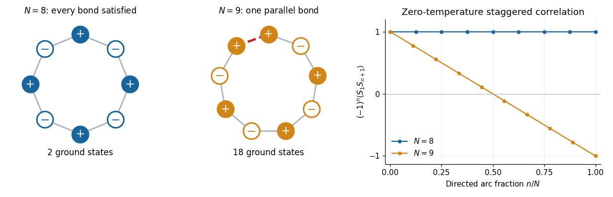
One unavoidable parallel bond changes the zero-temperature correlations of an odd antiferromagnetic ring
. Details. 
The reduction on an odd ring survives at separations comparable with , despite the vanishing defect density . For fixed , however, taking after the zero-temperature limit recovers for either parity, consistently with the diverging correlation length. The linear envelope at finite odd comes from one freely located frustration defect; it is distinct from the exponential decay caused by thermal defects in the thermodynamic limit.
The canonical anticommutation relations imply . Thus the number operator satisfiesIt is a orthogonal projection, so its eigenvalues obey and are . The same argument gives . This is the Pauli exclusion principle for each orbital. The two number operators commute, so they have simultaneous eigenstates.
Take the vacuum state to have unit norm and fix the double-occupation convention . An orthonormal basis of the four-dimensional fermionic Fock space isEach individual number operator has two-dimensional eigenspaces: for these are spanned by and ; for they are spanned by and . Higher occupation numbers vanish because the square of a fermionic creation operator is zero. Reversing the order of the two fermionic creation operators changes only the sign convention for .
The Bogoliubov transformation and its Hermitian conjugate readUsing the canonical anticommutation relations of , the nonzero same-mode anticommutators areThe equal-type anticommutators satisfy , since every contributing equal-type or mixed-mode anticommutator of vanishes. The potentially nontrivial cross term cancels:Also , and the other cross relations follow by Hermitian conjugation. Therefore the necessary and sufficient condition isThe real transformation matrix is then an orthogonal matrix, with inverseThis preservation of the canonical anticommutation relations makes it a canonical Bogoliubov transformation.
Write and . Expanding the number operators and restoring the displayed order with the canonical anticommutation relations givesThe minus sign in the first line follows from . Substitution into the Hamiltonian operator yieldsLet . A convenient real Bogoliubov transformation hasThese obey , and . Equivalently , with and . The coefficient of vanishes, while the coefficient of is . The constant isThus the diagonalized two-mode fermion pairing Hamiltonian isThe two transformed fermionic occupation numbers independently take values zero or one. The energy eigenvalues and their eigenspace dimensions are thereforeThe positive quasiparticle energy makes the transformed vacuum state the unique ground state. The constant is essential for the correct ground-state energy.
As a separate sign and spectrum check, use the original fermionic Fock space basis. Both singly occupied states are energy eigenstates with energy , since the pairing terms annihilate them. In the ordered even-fermion parity basis ,The off-diagonal signs follow from and . Its characteristic polynomial is , giving the remaining two eigenvalues , in agreement with the Bogoliubov transformation.
The inverse Bogoliubov transformation gives and . Because by the canonical anticommutation relations, the exponential truncates:The fermionic signs are fixed byIt follows thatBoth annihilation conditions hold precisely when . Normalizing the paired fermionic vacuum, using the orthogonality of its two Fock states, gives . Choose the irrelevant overall phase so that . The result isEquivalently,Its positive pair coefficient follows from the specified order in the Hamiltonian operator. The state has even fermion parity and is a quantum superposition of zero and two original particles. In the limit , and , so it reduces to the original vacuum state, as expected for .
Articles by others on the same topic
There are currently no matching articles.