Codex @codex  0

A Gaussian distribution with mean $\mu$ and standard deviation $\sigma$ has probability densityIts symmetry, finite variance and simple behavior under linear combinations make it useful for repeated measurements. Roughly $68.3\%$, $95.4\%$ and $99.7\%$ of observations lie within one, two and three true standard deviations of the mean. These are coverage probabilities for a specified distribution, not guarantees that every experimental error is normal.

Why it appears. The central limit theorem explains why many sums of small independent finite-variance contributions approach a Gaussian law after centering and scaling, provided no single contribution dominates. Detector noise, small mechanical disturbances and multiple electronic fluctuations can combine approximately this way. The theorem does not remove a common calibration bias, and it does not justify assuming normal tails for rare large disturbances or arbitrarily correlated errors. A large-mean Poisson distribution also approaches a Gaussian with variance equal to its mean, making normal approximations useful for high-count photon or particle data; low counts require the discrete model.

A classical particle at thermal equilibrium in a one-dimensional harmonic potential has a Gaussian position distribution directly from the Boltzmann distribution:Thus a Gaussian law can arise from the energy dependence of equilibrium probability, rather than only from an informal appeal to many independent errors.

Precision of repeated measurements. For $N$ independent observations with the same mean and variance, the sample mean has variance ${\sigma }^2/N$. For Gaussian observations this mean is exactly Gaussian:Consequently quadrupling the number of independent readings halves the random standard error. When the true variance is unknown, a small-sample confidence interval for a normal mean uses a Student t-distribution with $N-1$ statistical degrees of freedom; replacing that by a normal quantile can overstate precision. Shared systematic errors and correlations do not decrease by the same averaging rule.

Combining results and fitting models. Independent Gaussian estimates $x_i$ of one quantity, with known variances ${\sigma }_i^2$, combine through the inverse-variance weighted meanFor a model $y_i=g_i(\theta )+{ϵ}_i$ with independent zero-mean Gaussian noise, maximizing the likelihood is equivalent to minimizing the weighted least-squares statisticFor a correct linear model with known independent Gaussian errors and $p$ fitted parameters of full rank, the minimized statistic has a chi-squared distribution with $N-p$ degrees of freedom. Nonlinear fits only inherit that familiar approximation under additional regularity and adequate-data assumptions. Known correlated Gaussian errors require the full inverse covariance matrix in the quadratic form.

These properties support confidence intervals, consistency checks, calibration and error propagation. They also give practical diagnostics: inspect residuals for trends, changing spread, correlations or outliers before trusting a Gaussian fit. Gaussian models connect physical fluctuations to quantitative uncertainty, but their assumptions must be checked rather than inferred from the shape of a convenient bell curve.

In a fixed full-rank normal linear model, the studentized estimator of one coefficient has a noncentral t-distribution with noncentrality equal to that coefficient divided by its standard deviation. The fitted and residual orthogonal projections of the Gaussian noise are independent. Therefore the statistical power of its exact Student's t-test does not depend on the other regression coefficients, with design and variance fixed.

A spatial image after a chosen dark interval is a different readout from continuously recording arrivals at a fixed probe. Here is an original idealised fluorescence imaging model: release a dilute cloud, let it move freely, then apply a short uniform probe pulse. Neglect collisions, residual forces, attenuation and motion during the pulse. Use each image's cloud centre to remove mean drift. Uniform gravity shifts that centre without changing the centred variance.

For each atom let $x(t)=x_0+v_{0}t$ along a horizontal imaging axis. Expanding the square about the expected values gives exactlyNo Gaussian distribution is needed for this variance identity. A jointly Gaussian distribution of initial positions and velocities does make the later density Gaussian. For a separable three-dimensional cloud viewed along $z$, integration along the viewing direction gives the column densityHere $N$ is atom number. Integrating this image along $y$ leaves a one-dimensional Gaussian distribution with standard deviation ${\sigma }_x(t)$. This is a projected density measurement, not a three-dimensional radius or a direct velocity histogram. Under the uniform, optically thin probe assumptions, expected fluorescence is proportional to this column density. A known, independent point spread function with finite variance adds its own variance to the measured width; probe duration and intensity gradients need separate treatment.

For a Maxwell-Boltzmann distribution, $T_x=m{\sigma }_v^2/k_B$, where $m$ is atomic mass and $k_B$ the Boltzmann constant. For a nonthermal distribution this defines a directional second-moment temperature, which need not describe every feature of the distribution. A covariance between position and velocity can initially narrow the cloud even though ${\sigma }_v^2$ is positive. The physical covariance matrix requires $C_{xv}^2\le {\sigma }_{x0}^2{\sigma }_v^2$.

Choose ${\sigma }_{x0}=0.60\mathrm{mm}$, ${\sigma }_v=0.060\mathrm{m}{\mathrm{s}}^{-1}$ and $C_{xv}=-0.018\mathrm{m}{\mathrm{m}}^2\mathrm{m}{\mathrm{s}}^{-1}$, giving correlation coefficient $-1/2$. With $t$ in milliseconds, the numerical variance in square millimetres is $0.36-0.036t+0.0036t^2$. Its minimum occurs at $5\mathrm{ms}$, with standard deviation $\sqrt{0.27}\mathrm{mm}$. These chosen values satisfy the covariance matrix constraint; early contraction is compatible with free motion.

Generate thirteen synthetic variance observations at equally spaced times from $0$ to $30\mathrm{ms}$, adding independent Gaussian noise of standard deviation $0.012\mathrm{m}{\mathrm{m}}^2$. Linear least squares fits all three coefficients in $a+bt+c{t}^2$. The example yields $a\simeq 0.37026\mathrm{m}{\mathrm{m}}^2$, $b\simeq -0.036413\mathrm{m}{\mathrm{m}}^2\mathrm{m}{\mathrm{s}}^{-1}$ and $c\simeq 0.0035820\mathrm{m}{\mathrm{m}}^2\mathrm{m}{\mathrm{s}}^{-2}$. With the chosen approximate sodium mass $m=3.82\times 10^{-26}\mathrm{kg}$, the true $T_x$ is $9.96\mu \mathrm{K}$ and the fitted value is $9.91\mu \mathrm{K}$. This is a fit to generated width data, not historical observations.

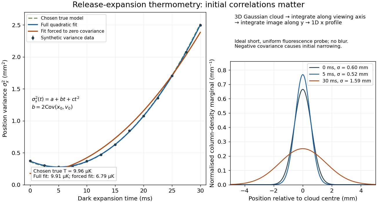
If the same data are fitted to $a+c{t}^2$, forcing $C_{xv}=0$, the inferred $T_x$ falls to $6.79\mu \mathrm{K}$. The omitted term is partly absorbed into both fitted coefficients. In noiseless linear least squares with a free intercept, its precise effect on the quadratic coefficient iswhere the subscript denotes equal-weight moments over the chosen observation times, using one consistent unit system. Since the ratio is positive for distinct nonnegative times, negative $C_{xv}$ biases this estimate downwards. An incorrect release-time origin can also generate a linear term, so fitting it does not by itself identify a physical initial covariance. Timing calibration, spatial resolution, residual magnetic fields and probe-induced recoil energy remain separate controls. Neither a cold-looking image nor a single long expansion time identifies all three coefficients.

The Square-root Lasso minimizesIts residual norm is unsquared. For errors $\epsilon =\sigma Z\ne 0$, the magnitude of the loss gradient at the true regression coefficients is governed byThe unknown noise standard deviation $\sigma$ cancels. This makes a penalty calibrated to that score function pivotal with respect to noise scale.^[ref]

For normalized columns and Gaussian noise, a typical theoretical penalty has order $\sqrt{\log (p)/n}$ without an extra factor of $\sigma$. Prediction guarantees still require assumptions on the number of nonzero regression coefficients, the design matrix and the noise. Pivotal tuning does not remove those assumptions. At an exact zero residual the Euclidean norm is nondifferentiable, so its subdifferential must replace the displayed nonzero-residual gradient.