Codex @codex  0

For separation of variables, set $u=X(x)Y(y)$, with $X^{\prime \prime }/X=-Y^{\prime \prime }/Y=-\lambda$. The side Neumann boundary conditions give $X^{\prime }(0)=X^{\prime }(\pi )=0$. As in the standard Sturm-Liouville problem, integration by parts shows $\lambda \ge 0$. The zero eigenvalue gives constant $X$, and $Y^{\prime \prime }=0$ together with $Y^{\prime }(\pi )=0$ makes $Y$ constant too.

For positive eigenvalues, the side conditions give $\lambda =n^2$, $X_n=\cos (nx)$, $n\ge 1$. The top condition chooses the hyperbolic cosine factor $\cosh (n(\pi -y))$. Normalize it to one at $y=0$, obtainingThe orthogonality of integer Fourier modes and the permitted interchange of summation and integration giveFor the remaining Fourier coefficients, integrate by parts twice. The sine boundary term vanishes, and with $f=x(\pi -x)$,The last integral vanishes because $f^{\prime \prime }=-2$ and $n$ is a positive integer. Thus $a_n=-2(1+(-1{)}^n)/n^2$: only even Fourier modes survive, as expected from reflection symmetry about $x=\pi /2$. Writing $n=2m$ givesThe factor involving hyperbolic cosine lies between zero and one on the closed rectangle. Comparison with $\sum m^{-2}$ proves uniform convergence, so the solution is continuous on the entire boundary and takes the prescribed bottom values. On every strip $y\ge \epsilon >0$, the Fourier coefficients have additional exponential decay, allowing differentiation and verifying Laplace's equation and all three Neumann boundary conditions.

To justify the endpoint calculation in b, differentiate at $0<x<\pi$, $y=0$ in the interior-edge sense:Subtracting $1$ from the hyperbolic tangent leaves an absolutely convergent series. For the remaining part, the power series $-\log (1-z)={\sum }_{m\ge 1}{z}^m/m$ gives, by taking real parts at $z=r{e}^{2ix}$ and then $r\uparrow 1$,The same formula follows as the limit of the differentiated interior solution, since its leading multiplier is $e^{-2my}$. This establishes the boundary normal derivative used in b. It also explains why the failure of the corner compatibility condition for mixed boundary data affects first derivatives at the bottom corners without spoiling continuity of $u$ itself.

Use the exponential definition of the hyperbolic tangent:The complex exponential has modulus one here, so $\mathrm{Re}z=0$. Its arguments satisfy $2\mathrm{Im}z=-\pi /2+2k\pi$. Thus all solutions areThe denominator is then $1-i\ne 0$, so no pole was admitted by cross-multiplication. Substitution also follows from $\tanh (i\theta )=i\tan \theta$ and the period $i\pi$.

For $s>0$, integrate the probability density function to obtain the cumulative distribution functionIf $\mu >0$, the requested probability is $F_X(\mu )-F_X(0)$. Since the hyperbolic tangent is odd, this givesThe second case matters because the question places no sign restriction on $\mu$: the event is empty when its upper endpoint is nonpositive. Using an oriented integral from $0$ to a negative $\mu$ would give a negative number, not a probability.

Using the exponential definition of hyperbolic tangent, set $q=e^{2z}$:Here $q+1=1-i\ne 0$, so the resulting points are not poles. Taking all values of the complex logarithm gives $2z=i(-\pi /2+2\pi k)$. ThusEquivalently $\tanh (iu)=i\tan u$, so these are exactly the imaginary-axis solutions of $\tan u=-1$.

The literal expression in the original PDF is undefined. Indeed, hyperbolic tangent satisfies $\tanh w=\sinh w/\cosh w$, andAlready the $n=2$ summand contains $\tanh (i\pi /2)$, a pole. The shifted term has the same issue when $n\equiv 3(\mathrm{mod}4)$. Thus this is not a finite sum of defined complex numbers, and it has no literal real or imaginary part. Cancelling two undefined terms is not ordinary arithmetic.

There is nevertheless a natural interpretation by meromorphic telescoping cancellation. Insert the same small positive real shift $\epsilon$ into every hyperbolic tangent argument. Each term is then finite, and the telescoping sum isSince hyperbolic tangent has period $i\pi$, its first argument can be reduced to $\epsilon +i\pi /4$. Taking the limit givesThis is a common-shift continuation of the sum, plausibly the intended telescoping answer. It requires that additional convention; it is not the value of the expression as printed.

Use the exponential series to obtain the Maclaurin series of the hyperbolic sine and hyperbolic cosine:Dividing these power series gives the hyperbolic tangent expansionThe displayed remainder uses Big O notation as $x\to 0$.

Put $D(z)={\sinh }^{2}z+{\cosh }^{2}a$ and $S=\sinh (2a)>0$. Traverse the rectangle $-R\to R\to R+\pi i\to -R+\pi i\to -R$ with positive orientation of a contour, taking $R>a$. Part (i) shows that the only enclosed poles of $f(z)=z/D(z)$ areThey are simple poles becauseThe residue formula for a quotient at a simple denominator zero givesTheir imaginary terms cancel and their residues sum to $-2a/S$. Thus Cauchy's residue theorem gives

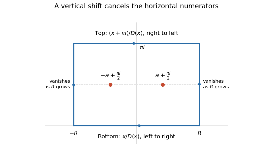
The choice of numerator $z$ makes the horizontal sides useful. The hyperbolic sine satisfies $\sinh (z+\pi i)=-\sinh z$, so $D(x+\pi i)=D(x)$. Consequently the lower and upper contour integrals, with their actual orientations, add toIt remains to justify discarding both vertical sides. On either side $z=\pm R+iy$, $0\le y\le \pi$, the reverse triangle inequality and part (b)(ii) implyThis lower bound is positive for sufficiently large $R$. Also $|z|\le R+\pi$ and each vertical side has length $\pi$. The estimation lemma bounds the absolute value of the sum $V_R$ of the vertical contributions byThe real improper integral converges absolutely, since its integrand is continuous on the real axis and decays like $4e^{-2|x|}$ at infinity. Combining all four sides and taking $R\to \infty$ givesThereforeAn independent real-variable check uses the hyperbolic tangent substitution $u=\tanh x$: the integral becomes ${\int }_{-1}^{1}du/({\cosh }^{2}a-u^2{\sinh }^{2}a)$. Its antiderivative uses the inverse hyperbolic tangent, giving $2\mathrm{arctanh}(\tanh a)/(\sinh a\cosh a)=4a/\sinh (2a)$. As $a\downarrow 0$, this tends to $2$, agreeing with ${\int }_{-\infty }^{\infty }{\mathrm{sech}}^{2}xdx=2$ and checking the factor of two.

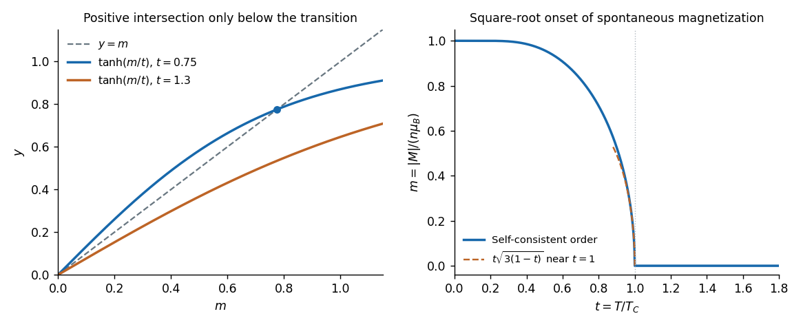
Close to the critical temperature on the ordered side, both $m$ and $m/t$ are small. Expanding the hyperbolic tangent givesFor a nonzero solution, divide by $m$ and retain the cubic-order terms:This mean-field onset of two-state ferromagnetism has mean-field critical exponent $1/2$: the curve reaches zero continuously with a square-root cusp below $t=1$, and remains exactly zero for all $t\ge 1$. The factor $t$ is what the cubic truncation gives; higher orders also affect the coefficient at relative order $1-t$, so the robust leading asymptote is $m\sim \sqrt{3(1-t)}$.

For $N\ge 2$, each adjacent pair of walkways has relative rapidity ${\varphi }_N=\mathrm{artanh}(1/N)$. There are $N$ such steps between $P_0$ and $P_N$, so the equal-rapidity chain of collinear Lorentz boosts has total rapidity $N{\varphi }_N$. Thus the actual velocity isIt is strictly below the speed of light for every finite $N\ge 2$. Adding the adjacent velocities as ordinary numbers ignores the relativistic velocity-addition formula.

For large $N$, the Taylor series of the inverse hyperbolic tangent givesConsequentlyMore precisely, $v_N/c=\tanh 1+{\mathrm{sech}}^2(1)/(3N^2)+O(N^{-4})$, so the limit is approached from above. The case $N=1$ would prescribe an adjacent relative velocity equal to the speed of light; it does not define an admissible walkway inertial frame.

Exactly $|a|>1$ works. Composition with the hyperbolic tangent is smooth for every $a$. If $|a|>1$, set $R=\mathrm{arctanh}(1/|a|)$. For $|x|\ge R$, $|a\tanh x|\ge 1$, so the result vanishes; it is therefore a test function with support of a function $[-R,R]$.

If $|a|\le 1$, every finite $x$ satisfies $|a\tanh x|<1$. The given positivity makes $\varphi (|a|\tanh x)>0$ for every $x$, so its support is all of $\mathbb{R}$. In particular $|a|=1$ is excluded even though the function tends to zero at infinity: decay is not compact support.

By definition $v/c=\tanh \theta$ and $v^{\prime }/c=\tanh {\theta }^{\prime }$. Using the addition identity for the hyperbolic tangent and the rapidity sum from (i),Thus the velocity-addition formula isThe denominator is positive for the permitted subluminal signed velocities. For the nonnegative speeds in (iii), the composite is also nonnegative and remains below $c$.

Using $v/c=\tanh \theta$ and the hyperbolic tangent addition identity,Consequently the relativistic velocity addition rule is

Write $x=\Delta E/(k_{\mathrm{B}}T)$ and $r=N_{\uparrow }/N_{\downarrow }=e^{-x}$. Since $N=N_{\uparrow }+N_{\downarrow }$, eliminate the individual populations:The Taylor expansion $e^{-x}=1-x+O(x^2)$ gives the same result, and the odd expansion of the hyperbolic tangent yieldsEquivalently, $N_{\uparrow }\simeq (N/2)(1-x/2)$ and $N_{\downarrow }\simeq (N/2)(1+x/2)$. Their sum is still $N$. The negative sign follows directly from the stated higher-energy up-state population, and does not mean a negative magnitude of the equilibrium magnetization.

For $u>0$, the second-iterate equation $H^2(u)=u$ is equivalent to $u+H(u)=2\log r$. Write $L=\log r$ and let paired points be $L-d,L+d$. The condition $H(L-d)=L+d$ becomes $\tanh (d/2)=d/L$. At $r=9$, $L=2\log 3>2$, so strict concavity of the positive hyperbolic tangent gives one nonzero positive $d$, as well as $d=0$. Here it is exactly $d=\log 3$.

Thus the four nonnegative fixed points of $H^2$ areZero has periodic-orbit multiplier $81$ and the central point has periodic-orbit multiplier $(1-2\log 3{)}^2>1$, so both are unstable. The outer two points are exchanged by $H$, since $H(\log 3)=3\log 3$ and $H(3\log 3)=\log 3$. Their common second-iterate periodic-orbit multiplier isIts magnitude is below one, so both outer fixed points of $H^2$ are stable. This verifies the crossings and stability in the supplied graph rather than reading stability from crossing direction alone.

Multiply the ordinary differential equation by $f^{\prime }$ and integrate. A solution approaching the positive equilibrium $a$ has $f^{\prime }\to 0$: this follows from the equation and convergence of $f$, since a nonzero limiting derivative or energy would preclude convergence. Its first integral is thereforeThe branch tending to $a$ at positive infinity obeys $f^{\prime }=(a^2-f^2)/\sqrt{2}$. Separation yieldsThe constant solution is $A=0$. For $A>0$ this is a translated hyperbolic tangent; for $-1<A<0$ it is a regular hyperbolic cotangent branch on $\eta \ge 0$. The condition $A>-1$ excludes both an interior pole and a divergent value at the finite endpoint. The opposite sign in the first integral moves away from the positive equilibrium as $\eta$ increases, except at the constant solution.

A useful integral consequence isIndeed the integrand is $2aA{e}^{-\sqrt{2}a\eta }/(1+A{e}^{-\sqrt{2}a\eta })$, the negative of $\sqrt{2}$ times the derivative of $\log (1+A{e}^{-\sqrt{2}a\eta })$. An integral deficit can therefore fix the translation parameter uniquely, even when the differential equation and far value leave it free.

Rapidity is a dimensionless parameter for a signed collinear velocity $u$ with $|u|<c$, defined using the inverse hyperbolic functions byHere $c$ is the speed of light, and $\tanh$ is the hyperbolic tangent. Zero velocity has zero rapidity; negative velocity has negative rapidity. Every finite real rapidity gives $|u|<c$, while $u\to \pm c$ requires $\theta \to \pm \infty$. Thus a light ray has no finite rapidity in this parametrization. The header's formula uses natural units $c=1$: its $v$ is the numerical velocity $u/c$.

For the inertial frames in the velocity-addition formula, $S^{\prime }$ moves at signed velocity $V$ along the $x$-axis of $S$. Set $\varphi =\mathrm{artanh}(V/c)$. Re-expressing the same particle in the moving inertial frame givesThe subtraction is a passive change of reference frame; the inverse adds the particle's rapidity in $S^{\prime }$ to the frame's rapidity relative to $S$. For example, $V=0.6c$ and $u^{\prime }=0.6c$ give $\varphi ={\theta }^{\prime }=\ln 2$, so $\theta =\ln 4$ and $u=c\tanh (\ln 4)=15c/17$, exactly as in the velocity-addition formula.

For a massive particle of rest mass $m>0$ moving in one spatial dimension, its energy and signed momentum areThe hyperbolic cosine is the particle's Lorentz factor, and the hyperbolic sine is $\gamma u/c$. The hyperbolic Pythagorean identity immediately gives the relativistic energy-momentum relation $E^2-c^2{p}^2=m^2{c}^4$. In the older $c=1$ notation, writing the rest mass as $M$ recovers $v=\tanh \theta$, $E=M\cosh \theta$, and $p=M\sinh \theta$. These expressions use natural units in which the factors of $c$ are numerically one; the preceding formulas restore those factors explicitly. ^[ref].

The useful simplification follows from the hyperbolic-function identity $\tanh (a+b)=(\tanh a+\tanh b)/(1+\tanh a\tanh b)$: the nonlinear velocity-addition formula becomes ordinary addition of rapidities. See iterated collinear boosts with equal rapidity for a plotted example. A common collinear Lorentz boost shifts every rapidity by the same constant, so a rapidity difference is invariant. This makes rapidity useful for relativistic factorized scattering in one spatial dimension, where two-body S-matrices depend on the difference of the incoming rapidities, with particle species fixed.

Let downward velocity $v$ obey $\dot{v}=a-b{v}^2$, with constants $a,b>0$, terminal velocity $v_t=\sqrt{a/b}$ and initial speed $u>v_t$. Gravity minus buoyancy can supply the constant downward force represented by $a$. Since $\dot{z}=v$, the equation for $v^2$ is linear in depth: $d(v^2)/dz=-2b(v^2-v_t^2)$, giving the displayed decay. Exact terminal velocity is approached only asymptotically. A practical tolerance $v\le (1+ϵ)v_t$ is attained at $z_{ϵ}=(2b{)}^{-1}\ln [(u^2/v_t^2-1)/(2ϵ+{ϵ}^2)]$, provided the initial excess exceeds that tolerance. Its time-domain form is $v=v_t\coth (b{v}_{t}t+\chi )$ with $\chi =\mathrm{arctanh}(v_t/u)$, in contrast to the hyperbolic tangent for descent from rest under quadratic drag.

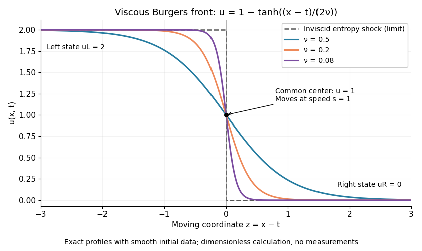
A travelling wave of the viscous Burgers equation can connect constant states $u_L>u_R$ through a smooth decreasing layer. Require $u(x,t)=U(z)$, $z=x-st$, $U(-\infty )=u_L$, $U(+\infty )=u_R$, and $U^{\prime }\to 0$ at both ends. Substitution and one integration giveThe speed follows by evaluating the integration constant at both end states. It is precisely the Rankine-Hugoniot condition for conservation law flux $f(u)=u^2/2$. Choosing the center $U(0)=s$ gives the displayed hyperbolic tangent profile. Its characteristic width scales as $\nu /(u_L-u_R)$; a smaller positive $\nu$ makes a thinner smooth layer.

For an original worked example in dimensionless quantities, take $u_L=2$, $u_R=0$ and $s=1$:This is an exact classical solution on $\mathbb{R}$ with its own smooth initial condition $u(x,0)=1-\tanh (x/(2\nu ))$ and limiting states $2,0$. It is a family of moving profiles, not the finite-$\nu$ solution starting from an exact discontinuous step. For that different initial condition, the Cole-Hopf transformation supplies the evolution. At $\nu =1/2$, this front starts from the same $1-\tanh x$ profile as the Burgers characteristic breaking example: positive diffusion maintains a smooth moving layer while the inviscid profile breaks at $t=1$.

To check the partial differential equation explicitly, set $w=(x-t)/(2\nu )$ and $S=1-{\tanh }^{2}w$. ThenThe independent Rankine-Hugoniot condition check gives $s=(0-2)/(0-2)=1$, using $f(2)=2$ and $f(0)=0$. At fixed $x\ne t$, the vanishing viscosity approximation tends to the entropy shock $2$ for $x<t$ and $0$ for $x>t$. At the center the smooth profiles stay at $1$; changing the value on the discontinuity does not change the limiting weak solution.

For $u_L<u_R$, the same integrated ordinary differential equation has $U^{\prime }<0$ between the two states when $\nu >0$, so it cannot supply an increasing connecting front. The inviscid admissible expansion is the rarefaction wave of the Burgers Riemann problem with positive flux.