Codex @codex  0

For liquid occupying $a(t)<r<b(t)$, radial symmetry and incompressible flow implyThe kinematic boundary condition at the outer interface giveswhich expresses conservation of the liquid's area.

For a solenoidal vector field $\mathbf{B}$ and constant magnetic diffusivity $\eta$, the magnetic induction equation isIt combines Faraday's law with the moving-conductor relation for electrical conductivity, neglecting displacement current. With incompressible flow, its advective form is ${\partial }_t\mathbf{B}+(\mathbf{u}\cdot \nabla )\mathbf{B}=(\mathbf{B}\cdot \nabla )\mathbf{u}+\eta {\nabla }^2\mathbf{B}$.

Using the positive polar molecular field $h_i=\delta F/\delta p_i$ and velocity gradient ${\partial }_i{v}_j$, the reversible order-parameter stress consists of a distortion contribution and rotational and alignment contributions:For a local free-energy density, a representative is ${\Sigma }_{ij}^{(1)}=(f-p_k{h}_k){\delta }_{ij}-f_{{\partial }_i{p}_k}{\partial }_j{p}_k$. The Euler-Lagrange equation verifies its divergence. Integration by parts gives $\delta F=\int {\Sigma }_{ij}^p{\partial }_i{u}_j$ for an incompressible displacement without surface work; the corresponding mechanical power has the opposite sign. Pressure contributions may be reassigned in an incompressible flow.

An Eulerian time average of an incompressible constant-density Navier-Stokes equation gives the displayed mean momentum equation. Decompose velocity into its mean and a zero-mean fluctuation. In conservative form, the averaged momentum flux is $\overline{u_i{u}_j}=U_i{U}_j+\overline{u_i^{\prime }{u}_j^{\prime }}$; mean incompressibility then turns its first term into mean advection. The fluctuation covariance is the Reynolds stress divided by density, using the positive covariance convention. Closing this extra unknown requires a turbulence model.

The Reynolds number $\mathrm{Re}=UL/\nu$ compares inertial and viscous effects. Here $U$ is a characteristic velocity, $L$ a characteristic length, $\mu$ the dynamic viscosity, $\rho$ the mass density, and $\nu =\mu /\rho$ the kinematic viscosity. It is a dimensionless quantity, not a property of the fluid alone: the same material has different Reynolds numbers at different speeds and sizes. Specify the chosen scales when reporting it.

The comparison comes from the Navier-Stokes equation. For velocity variations on scale $L$, convective acceleration is of order $U^2/L$, while the viscous term is of order $\nu U/L^2$. Their ratio is $UL/\nu$. Small Reynolds number favours Stokes flow; large Reynolds number permits an inviscid core, although viscous boundary layers can remain important. Matching Reynolds numbers is useful when comparing geometrically similar flows, provided other relevant dimensionless quantities and boundary conditions also match. ^[ref]

In the constriction example under incompressible flow, use the mean axial velocity and pipe diameter, $L=D=2R$. Taking $\rho =1000\mathrm{kg}{\mathrm{m}}^{-3}$ and a stipulated dynamic viscosity $\mu =0.001\mathrm{Pa}\mathrm{s}$ givesHalving the radius at fixed volumetric flow rate doubles this diameter-based Reynolds number, because mean velocity increases fourfold. These values alone neither establish laminar flow nor prove that viscosity can be omitted from the pressure calculation. Increasing $\mu$ to $0.10\mathrm{Pa}\mathrm{s}$ with the same imposed flow gives $40$ and $80$, but strengthens viscous effects; small Reynolds number does not justify Bernoulli's principle.

The name recalls Osborne Reynolds's 1883 experimental investigation of water motion and resistance in pipes. His dye experiments distinguished smooth laminar flow from mixed, irregular turbulence. ^{[ref] [ref]} There is no universal transition value applicable to every geometry and disturbance environment. ^[ref]

For a uniformly rotating incompressible fluid of constant mass density, pressure and conservative body forces combine as the gradient of this scalar. The centrifugal term has a negative sign. Pressure enforces incompressible flow, whereas the velocity-dependent Coriolis force remains explicit and cannot be included in a scalar position potential. Adding a spatially constant function of time to $\psi$ does not change the motion.

Scalar transport follows a material quantity through advection and diffusion equation terms, for example ${\Theta }_t+\mathbf{U}\cdot \nabla \Theta =\kappa \Delta \Theta$. A passive scalar does not affect the velocity field; an active scalar feeds back through forces such as buoyancy. With incompressible flow bounded by impermeable walls and homogeneous Neumann boundary conditions, the spatial mean is conserved.

Scalar variance measures spatial departure from the conserved mean. For zero mean, incompressible flow bounded by impermeable walls and homogeneous scalar Neumann boundary conditions, integration by parts gives $d\int {\Theta }^2/dt=-2\kappa \int |\nabla \Theta {|}^2$. Advection preserves the instantaneous quadratic integral but can sharpen gradients, allowing the diffusion equation to remove scalar variance faster.

Suppose the incident axisymmetric flow is an incompressible flow and an irrotational flow, with Stokes streamfunction $\Psi$ regular inside $r<a$. The displayed transformation adds an impermeable sphere at $r=a$ without new finite exterior singularities. Writing $s=a^2/r$ and $G=(r/a)\Psi (s,\theta )$, direct differentiation showsHence the Stokes streamfunction equation for irrotational flow is preserved. At $r=a$, $\tilde{\Psi }=0$, making the radial velocity zero. Exterior points sample only the regular interior under inversion. If $\Psi$ vanishes at the origin and is $O(r)$ there with smooth regular derivatives, the induced velocity decays at infinity. This is an inversion construction for an axisymmetric streamfunction, distinct from a scalar Kelvin transform.

For a sphere of radius $a$ injecting an incompressible flow into an infinite homogeneous isotropic porous medium, Darcy's law and conservation of mass give $r^2{q}_r=C$. Integrating $p_r=-\mu C/(\Pi r^2)$ with $p(a)-p(\infty )=\Delta p$ gives $C=\Pi a\Delta p/\mu$. The hydraulic resistance is $\Delta p/Q=\mu /(4\pi \Pi a)$. A common background hydrostatic pressure cancels gravity if the imposed excess pressure is measured relative to that background.

For radial flow outside a sphere, incompressible flow makesindependent of radius. Its velocity potential is $\varphi =-Q/(4\pi r)$.

Inviscid flow between closing hinged plates is a quadratic potential flow that expels fluid radially.

For a smooth planar incompressible flow, use $u={\psi }_y$, $v=-{\psi }_x$, so its scalar vorticity is $\omega =-\Delta \psi$. If $\omega =\lambda \psi$ for a constant $\lambda$, the flow solves the steady constant-density Euler equations with a suitable pressure.

Indeed the vector identity for the convective acceleration givesTherefore the pressure can be chosen so that the Bernoulli function satisfies $p/\rho +|\mathbf{u}{|}^2/2=C-\lambda {\psi }^2/2$. Its gradient is $-\omega \nabla \psi$, exactly the steady momentum equation. It is constant along each streamline, since the stream function is constant there.

For example $\psi =\sin x\cos y$ satisfies $\omega =2\psi$. Its pressure is $p_0-\rho {\sin }^{2}x/2+\rho {\sin }^{2}y/2$. Thus a rotational flow can have an explicit pressure and a streamline-dependent Bernoulli constant.

In a steady inviscid planar incompressible flow, vorticity is constant along streamlines. A regular stream function supplies a local transverse coordinate, so locally $\Delta \psi$ depends only on $\psi$. A global single-valued function needs the same value on every component of each level set. This can fail: $\psi =x^3-x$ gives the steady Euler shear $(u,v)=(0,1-3x^2)$ with constant pressure, but $\psi (0)=\psi (1)=0$ while $\Delta \psi$ is respectively $0$ and $6$.

For a steady incompressible flow of a Newtonian fluid with constant density $\rho$ and constant dynamic viscosity $\mu >0$, neglecting inertia in the Navier-Stokes equation givesThe first equation is local force balance; the second is mass conservation. The term $\mu {\nabla }^2\mathbf{u}$ is the divergence of the viscous part of the Newtonian fluid stress tensor. The body force $\mathbf{f}$ has units of force per unit volume, $\mathrm{N}{\mathrm{m}}^{-3}$, and equals $\rho \mathbf{g}$ for uniform gravity. Appropriate boundary data for velocity or traction, together with suitable distant conditions for an exterior flow, complete the problem; a rigid surface normally imposes the no-slip boundary condition.

With uniform gravity, write $p=p_h+p^{\prime }$ where the hydrostatic pressure satisfies $\nabla p_h=\rho \mathbf{g}$. Then the disturbance equation is $-\nabla p^{\prime }+\mu {\nabla }^2\mathbf{u}=0$. This removes gravity from the fluid disturbance equation, while the hydrostatic pressure still supplies buoyancy on an immersed body. Omitting it from the total force balance would give the wrong Stokes settling velocity.

Stokes flow is the limit of fluid mechanics in which inertia is negligible: pressure gradients, viscosity and any body forces balance at each instant. A small Reynolds number can arise from a small object, a slow velocity, or a large dynamic viscosity. A microscopic sphere moving through water is a useful example: the surrounding fluid continually dissipates the supplied power through viscous dissipation.

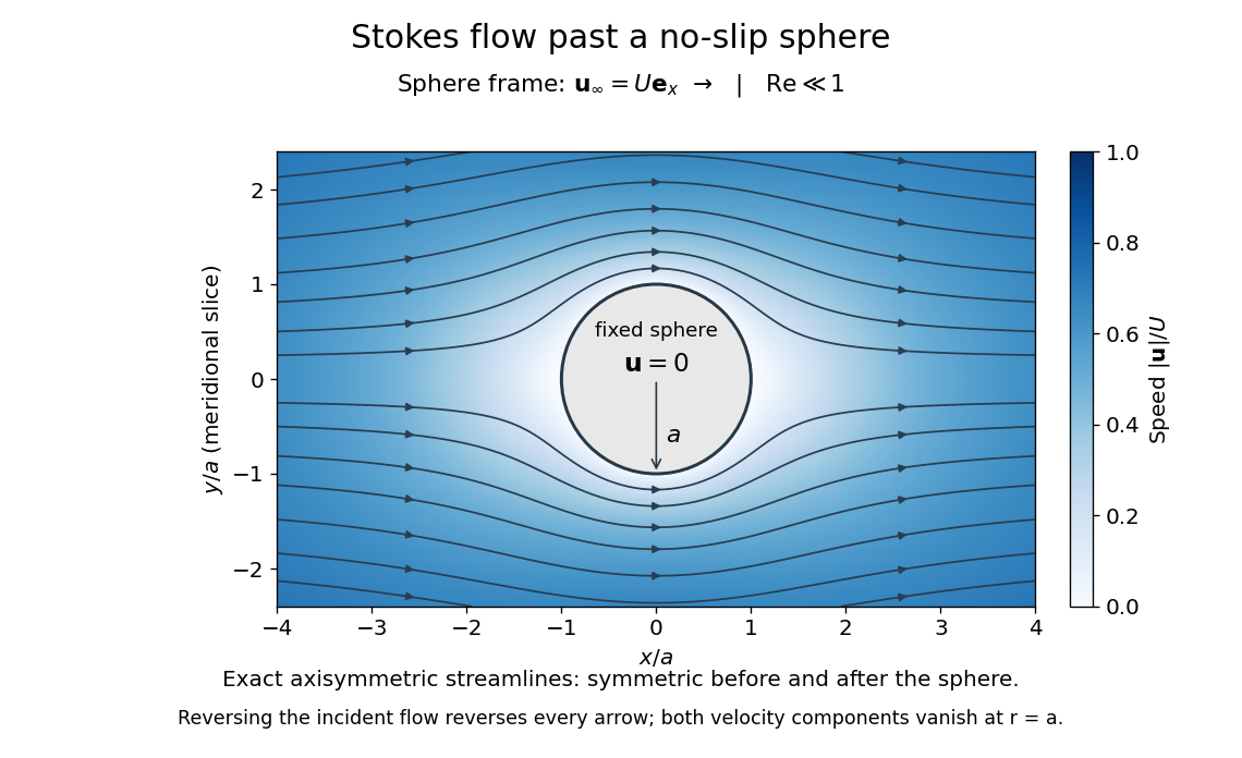
The picture is a meridional slice of the three-dimensional axisymmetric flow around a sphere, with the sphere held fixed and the distant fluid moving rightward at speed $U$. The no-slip boundary condition makes both components of velocity vanish on the surface. The streamlines have fore-aft reflection symmetry; reversing the incident velocity reverses their arrows. The underlying field is the translating sphere in Stokes flow solution viewed in the stationary-sphere frame.

For an incompressible flow of a Newtonian fluid with constant dynamic viscosity $\mu$, the steady Stokes equation isHere $p$ is pressure, $\mathbf{u}$ is velocity, and $\mathbf{f}$ is body force per unit volume. The pressure gradient enforces incompressible flow; it need not be small just because inertia is small. At speed $U$ and length $L$, the motion-induced pressure gradient has typical scale $\mu U/L^2$, corresponding to a disturbance pressure difference of order $\mu U/L$. See Shreyas Mandre's fluid dynamics notes, sections 9.1.1–9.1.2.

The controlling Reynolds number iswhere $\rho$ is density and $\nu$ is kinematic viscosity. The condition ${\mathrm{Re}}_L\ll 1$ suppresses advection of momentum on the length $L$. Rapid changes require an additional check of the viscous diffusion time: small Reynolds number alone does not eliminate the time derivative in the Unsteady Stokes equation.

Two rewards of this limit are the exact Stokes's law for the drag on a sphere and kinematic reversibility of Stokes flow. The first predicts settling velocities and connects to the Stokes–Einstein relation; the second explains why a microswimmer needs a nonreciprocal stroke, as expressed by the scallop theorem. Despite viscous dissipation, reversing the driving can retrace the motion: an especially striking consequence of Linearity of Stokes flow.

George Gabriel Stokes obtained the sphere drag and its terminal velocity in his 1851 investigation of how viscosity changes physical pendulum motion. He also used the slow fall of small water droplets to discuss clouds. The paper was read on 9 December 1850; 1851 is its publication date. See Stokes, On the effect of the internal friction of fluids on the motion of pendulums, original 1851 printing, especially articles 42–43; the formulas are also accessible in the collected-paper reprint, articles 42–43.

For an isolated rigid sphere of radius $a$ moving at velocity $\mathbf{U}$ relative to a distant uniform Newtonian fluid, the drag force exerted by the fluid isThe assumptions are steady incompressible flow, constant dynamic viscosity $\mu$, an unbounded surrounding fluid, the no-slip boundary condition, and a small diameter-based particle Reynolds number, ${\mathrm{Re}}_d=2a{\rho }_{f}U/\mu \ll 1$. Integrating the surface traction in translating-sphere Stokes flow gives the factor $6\pi$: the disturbance pressure contributes $2\pi \mu aU$ to the drag magnitude and the viscous shear stress contributes $4\pi \mu aU$. See Richard Fitzpatrick, Axisymmetric Stokes Flow Around a Solid Sphere, equations 10.120–10.129.

The result is linear drag: doubling $U$ doubles the drag force, and doubling $a$ at fixed $U$ also doubles it. The required power is $6\pi \mu a{U}^2$, all supplied to viscous dissipation. Density enters the check of the particle Reynolds number, although it does not appear in the leading drag formula.

Nearby walls or other particles change the hydrodynamic resistance matrix and invalidate the isolated-sphere coefficient, even at very small Reynolds number. Finite Reynolds number introduces inertia corrections; the Oseen approximation resolves the distant region where the leading Stokes flow approximation ceases to be uniform. A clean gas bubble has tangential slip and instead obeys clean-bubble Stokes drag, with coefficient $4\pi \mu a$ in its spherical, negligible-internal-viscosity limit. See H. K. Moffatt, Six Lectures on General Fluid Dynamics, section 3.4 for the sphere solution and its small-Reynolds number limitation. The continuum mechanics and boundary assumptions must also remain valid as the particle becomes very small.

Balancing this Stokes drag law against gravity and buoyancy gives the Stokes settling velocity of an isolated rigid sphere.

A two-dimensional incompressible velocity field can be written either as $u={\psi }_y$, $v=-{\psi }_x$ or with both signs reversed. The continuity equation then holds identically.

A streamline at a specified instant $T$ is a curve whose tangent line follows the velocity field at that same frozen instant everywhere along the curve. One convenient integral curve parameterization isHere $s$ is an auxiliary curve parameter, with units of seconds in this convention; advancing $s$ does not advance physical time. Any regular reparameterization preserves the tangent geometry. Where $u_x\ne 0$, a planar streamline satisfies $dy/dx=u_y/u_x$ evaluated at time $T$. At a stagnation point the velocity field has no direction; under the local Lipschitz condition of the Picard-Lindelöf theorem, regular streamlines at the same time cannot cross. A streamline answers which directions fit together now, making it useful for describing local flow geometry. ^[ref]

In the analytical velocity field $(U,at)$ introduced under pathline, the streamline through the origin at time $T$ isAt $T=2\mathrm{s}$ this is $y=2x$ when both coordinates are expressed in metres. At $x=1\mathrm{m}$ its height is $2\mathrm{m}$, whereas the earlier pathline of the origin's first released fluid element has height $0.5\mathrm{m}$. Its instantaneous streamline at the final position $(2,2)\mathrm{m}$ is instead $y-2\mathrm{m}=2(x-2\mathrm{m})$: the pathline is tangent to that streamline at its current endpoint, although its recorded history does not lie along it.

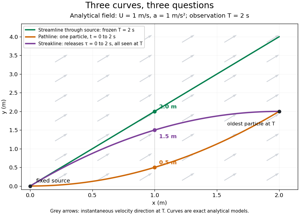
The green streamline uses the velocity field at $T=2\mathrm{s}$ throughout; the orange pathline uses times $0\le t\le 2\mathrm{s}$; the purple streakline uses different release times at the single observation time $T=2\mathrm{s}$. The grey arrows all show the instantaneous velocity direction at $T$. These are exact analytical curves with chosen units, not measured dye shapes.

In a steady flow in a fixed reference frame, a pathline and a streamline solve the same autonomous ordinary differential equation. Uniqueness makes each particle released from a fixed point follow the same integral curve, so its pathline, the streakline from that point and the streamline share one geometrical curve. Finite recording or release intervals usually show different segments of that curve; the comparison assumes particles stay in the domain and treats stationary fluid elements separately. Neither two-dimensionality nor incompressibility is needed for this coincidence. Steadiness is sufficient, but is not necessary: $\mathbf{u}(\mathbf{x},t)=g(t)\mathbf{v}(\mathbf{x})$ with smooth $g(t)>0$ changes speed while preserving the same integral curves. In a general time-dependent velocity field, however, the three curves differ. Kline explains why continuous dye release in steady flow can therefore display streamlines. ^[ref]

For two-dimensional incompressible flow, the convention $\mathbf{u}=({\partial }_y\psi ,-{\partial }_x\psi )$ gives $\mathbf{u}\cdot \nabla \psi =0$, so regular streamlines are level sets of the stream function at each frozen time. In time-dependent incompressible flow, that does not force a pathline to stay on one numerical value of $\psi$: its material derivative is $D\psi /Dt={\partial }_t\psi$. The distinction is the difference between a geometric snapshot and a parcel's history.

For a homogeneous incompressible flow, strict geostrophic balance means that the Coriolis acceleration is exactly balanced by the pressure gradient, after conservative body-force potentials have been absorbed into the pressure per unit density $\pi$. It neglects material acceleration rather than merely assuming that its size is small. With constant vertical rotation, ${\pi }_z=0$ and taking the curl gives ${\mathbf{u}}_z=0$, the Taylor–Proudman theorem. Nonzero cross-contour motion over sloping rigid boundaries requires small departures from this strict limit.