Codex @codex  0

For Brownian motion, write the later maximum as $B_b+Z+H$, where $Z=B_c-B_b$ has a nondegenerate normal distribution and $H={\sup }_{0\le u\le d-c}(B_{c+u}-B_c)$. The independent increments make $Z$ independent of the earlier history and of $H$. Conditional on those two objects, equality of the two maxima prescribes one value of $Z$, an event of probability zero. This argument uses the positive gap $c-b$ and does not assume independence of the two absolute maxima.

For standard Brownian motion started at zero, the strict first-passage times form a subordinator in the level parameter $a$. The Strong Markov property gives independent increments and stationary increments; the strict inverse of the continuous running maximum has càdlàg paths. The Brownian first-passage Laplace transform gives Laplace exponent $\Phi (\lambda )=\sqrt{2\lambda }$, so the process is strictly stable of index $1/2$. Choosing the non-strict hitting times preserves each fixed-level law but generally loses right continuity at random levels, as in the fixed-level versus simultaneous Brownian passage-time equality.

Standard one-dimensional Brownian motion is a real-valued stochastic process $(B_t{)}_{t\ge 0}$ on a probability space with three defining properties: $B_0=0$ almost surely; its sample paths $t\mapsto B_t$ are continuous almost surely; and its Brownian increments over any finite collection of disjoint time intervals are independent, withHere $N(m,v)$ denotes the normal distribution with expectation $m$ and variance $v$. The alternative symbol $W_t$ denotes the same kind of stochastic process. Continuity is a simultaneous statement about an entire sample path, rather than a separate assertion at each fixed time. Relative to its natural Brownian filtration, a future Brownian increment is independent of all observations up to its starting time.

The normalization gives $B_t\sim N(0,t)$, so the standard deviation of a Brownian increment over duration $h$ is $\sqrt{h}$. For $h=1$, $0.01$, and $0.0001$, the corresponding standard deviations are $1$, $0.1$, and $0.01$. Time becoming one hundred times shorter makes typical displacement ten times smaller. Brownian scaling expresses this rule for the whole stochastic process, while the Brownian covariance kernel describes how positions at different times remain related despite independent increments.

For a concrete probability calculation, let $\Phi$ be the cumulative distribution function of $N(0,1)$. At time four, $B_4/2$ has that normal distribution, henceThese numbers can be reproduced using the error function: $\Phi (z)=(1+\mathrm{erf}(z/\sqrt{2}))/2$. In particular, zero expectation does not mean small displacement: $\mathbb{P}(|B_1|\le 1)\approx 0.6826894921$, but the same fixed interval contains only about $38.3\%$ of the probability at time four.

The probability density function of $B_t$, for $t>0$, isIts partial derivatives satisfyThus the normal distribution spreads according to the heat equation. Starting at a fixed position $x_0$ replaces $x$ by $x-x_0$. This is a useful bridge between individual random trajectories and the deterministic evolution of their probability density function: the same Brownian motion provides both descriptions.

Physical diffusion uses its own scale. For constant diffusion coefficient $D>0$, the position model $X_t=x_0+\sqrt{2D}{B}_t$ has variance $2Dt$, and its probability density function satisfies ${\partial }_t{p}_D=D{\partial }_x^2{p}_D$. For example, $D=0.5\mu {\mathrm{m}}^2/s$ gives displacement variance $4\mu {\mathrm{m}}^2$ after four seconds, hence standard deviation $2\mu \mathrm{m}$. Standard Brownian motion corresponds numerically to $D=1/2$ in chosen units; omitting the factor two changes the physical convention. Einstein's 1905 paper relates diffusion to the mean squared displacement in precisely this convention. ^[ref]

Continuity does not supply a smooth physical velocity. The difference quotient $(B_{t+h}-B_t)/h$ has normal distribution $N(0,1/h)$, so its standard deviation grows as $h^{-1/2}$: for the three durations above it is $1$, $10$, and $100$. This calculation motivates the nowhere differentiability of Brownian motion, but it alone is not a proof of the simultaneous assertion at every time. The theorem says that, with probability one, no finite derivative exists anywhere along the sample path. A drawn polygon only displays a finite grid; its straight segments cannot establish this theorem. See Theorem 7.1.6 in Probability: Theory and Examples (fifth edition) by Rick Durrett.

For physical particles, Brownian motion is a model of position on suitable observation scales. It does not claim that microscopic velocity is a derivative of this idealized path. Einstein explicitly restricts his assumption of independent increments to intervals that are not too short. ^[ref]

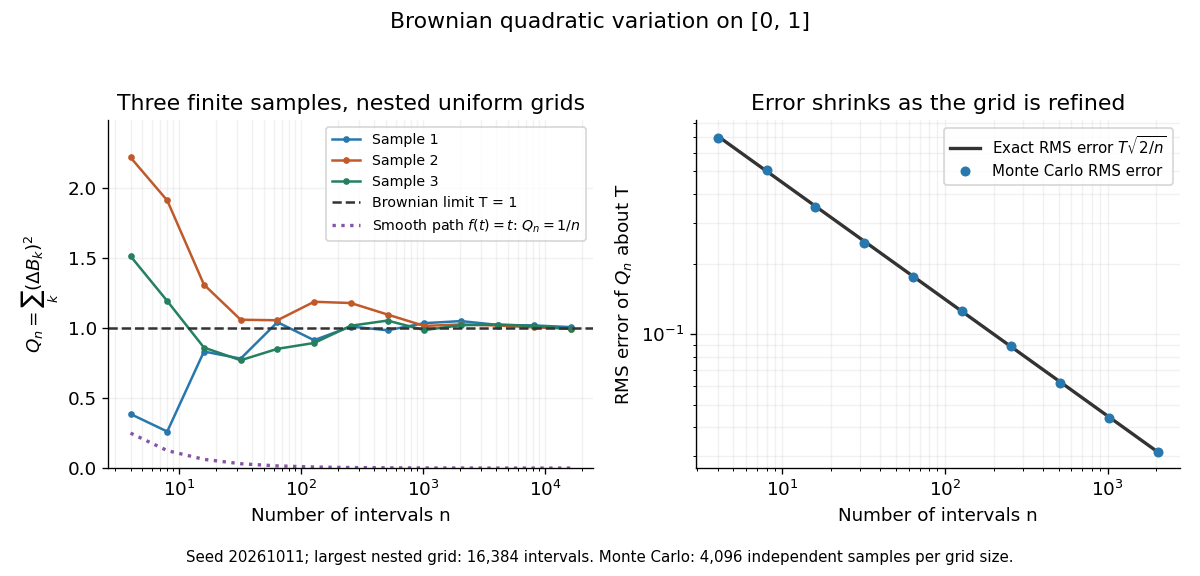
Another way to measure the roughness is quadratic variation. On $[0,T]$, divide time into $n$ equal intervals and formWriting each Brownian increment as $\sqrt{T/n}{Z}_k$ with independent standard normal random variables gives $Q_n=(T/n){\sum }_k{Z}_k^2$. Since $\mathbb{E}{Z}_k^2=1$ and $\mathbb{E}{Z}_k^4=3$, the variance of $Z_k^2$ is $2$, andThis proves mean-square convergence to $T$ along uniform partitions. For $T=2$ and $n=100$, the expectation is $2$, the variance is $0.08$, and the root mean square of the error is $\sqrt{0.08}\approx 0.2828427125$. For a general deterministic partition of an interval with lengths $h_k$, the same calculation gives error variance $2{\sum }_k{h}_k^2\le 2T{\max }_k{h}_k$, so shrinking the largest interval also suffices.

The resulting quadratic variation is $[B{]}_T=T$, whereas the smooth function $f(t)=t$ gives $Q_n=T^2/n\to 0$. This difference explains why the ordinary rules of calculus need the second-order correction in the Itô formula. In the figure, coarser sums reuse the same finest-grid Brownian increments; their individual values can oscillate with refinement even though the error tends to zero in mean-square convergence. Refining a fixed interpolating polygon forever would instead give zero quadratic variation, so the finite-grid illustration must not be confused with the limiting Brownian motion.

Historically, Brown's 1828 report describes microscopic observations made in 1827, starting with particles released from pollen and extending to inorganic materials; this challenged an explanation based solely on living matter. His observations and the later mathematical model are distinct contributions. ^[ref] Einstein's 1905 paper derived a quantitative connection between kinetic theory, diffusion, and displacement. ^[ref] Wiener's 1923 Differential-Space developed integration on spaces of paths, a foundation for Wiener measure; it also acknowledges earlier work and his own previous papers. These dates mark documented contributions rather than an assertion that each subject had a single discoverer. ^[ref]

For every fixed mesh $1/k$, independent increments with the normal distribution imply increments of absolute value greater than one occur infinitely often almost surely, by the second Borel-Cantelli lemma. A countable intersection over $k$ contradicts uniform continuity on $[0,\infty )$.

A càdlàg modification of a stochastic process is a modification of a stochastic process whose paths are càdlàg on one event of probability one. Equality almost surely at every separately fixed time does not imply indistinguishability of stochastic processes when the original process lacks path regularity. A stochastic process starting at zero, with independent increments, stationary increments, and stochastic continuity, has a càdlàg modification and is a Lévy process under the intrinsic definition.

The circle-average process of a zero-boundary Gaussian free field in the unit disc has the law of a constant multiple of Brownian motion. It is a continuous centered Gaussian process with stationary increments and independent increments and starts at zero.

Suppose Lévy processes $X^n$ converge to $X$ in probability at every fixed time, andThen $X$ starts at zero, has independent increments and stationary increments, and has stochastic continuity. Finite increment vectors inherit their independent laws by convergence in distribution; the near-zero estimate supplies continuity at zero. Hence $X$ has a càdlàg modification that is a Lévy process. The hypotheses alone cannot assert that the original version has càdlàg paths.

For a parabolic wave equation driven by longitudinal Gaussian white noise with transverse covariance kernel $B$, the mean envelope obeys ${\partial }_{x}m=i{\Delta }_{\perp }m/(2k_0)-\gamma m$. This closure requires independent increments in the longitudinal direction; statistical homogeneity and one-point Gaussian distributions alone are insufficient.

A process has conditionally symmetric increments if, for all deterministic $s\le t$ and bounded measurable $g$,Equivalently, the conditional characteristic function of every increment is invariant under changing the sign of its argument. This property is stronger than unconditional symmetry and is different from independent increments. It supplies identities between positive and negative exponential terminal martingales.

Conditionally on an ${\mathrm{SLE}}_{\kappa }$ initial segment through time $t$, mapping out that segment by $g_t-U_t$ turns the future into an independent ${\mathrm{SLE}}_{\kappa }$ in $(\mathbb{H},0,\infty )$. This follows because its driving function is $U_{t+s}-U_t$, and Brownian motion has stationary increments and independent increments.

For a nondecreasing process $A$ with stationary increments and independent increments, suppose $\mathbb{E}{e}^{\theta A(t)}=e^{t\Lambda (\theta )}$. If $\Lambda (\theta )\le C\theta$, then $e^{\theta (A(t)-Ct)}$ is a nonnegative supermartingale. Applying the maximal inequality for a nonnegative supermartingale up to time $T$ and then letting $T\to \infty$ givesThe stationary workload of a stable queue fed by $A$ has this supremum distribution, using the past input and stationary increments and independent increments. For independent flows, the constraint is ${\sum }_j{a}_j(\theta )\le C$, where $a_j(\theta )={\Lambda }_j(\theta )/\theta$ is the long-time effective bandwidth. The result bounds a continuous-time supremum directly; a one-time Chernoff bound by itself does not do that.

Independent increments and stationary increments make a Lévy process's characteristic functions multiplicative in time. Together with continuity of Lévy characteristic functions and the value one at time zero, this forces an exponential. A continuous local complex logarithm is additive: its failure of additivity would be a continuous integer multiple of $2\pi i$, hence zero. The Cauchy functional equation and subdivision then give the exponential at every time. This construction of the characteristic exponent of a Lévy process precedes the Lévy–Khintchine formula describing the exponent's possible form.

With the convention $\mathbb{E}{e}^{iu{X}_t}=e^{t\psi (u)}$, this complex process is a martingale for each real $u$. Its absolute value is the deterministic finite number $e^{-t\mathrm{Re}\psi (u)}$. Conditioning on the past at time $s$ and using independent increments multiplies $e^{iu{X}_s-t\psi (u)}$ by $e^{(t-s)\psi (u)}$, giving $M_s^u$. Under the opposite exponent convention the sign of the compensating term reverses.

In a classical risk model, an adjustment coefficient $R$ makes $\lambda (M_X(R)-1)-cR=0$. The random-sum transform identity and independent increments show that $\mathbb{E}[Z_t\mid {\mathcal{F}}_s]=Z_s$. This nonnegative martingale starts at one. At the ruin stopping time $\tau$, $Z_{\tau }>e^{Ru}$. Applying the optional stopping theorem only to $\tau \wedge t$ yields $\mathbb{P}(\tau \le t)\le e^{-Ru}$; passage to increasing horizons proves the Lundberg inequality without an unjustified expectation identity at an unbounded stopping time.

An increment of a real- or vector-valued stochastic process is the difference $X_t-X_s$ between its values at two times $s<t$. A random walk accumulates its one-step increments; a Poisson process has nonnegative integer increments counting arrivals in $(s,t]$. A process can have independent increments even though its values at different times are dependent.

A stochastic process has independent increments when, for every $t_0<t_1<\cdots <t_k$, the random variables $X_{t_1}-X_{t_0},\dots ,X_{t_k}-X_{t_{k-1}}$ are independent. Adjacent intervals are allowed: each increment represents the change after its left endpoint up to its right endpoint. A Poisson process, Brownian motion, and a random walk with independent steps have this property. Their values at different times need not be independent: for a fair simple random walk on the integer line, $\mathrm{Cov}(S_m,S_n)=\min (m,n)$ because both positions contain the same first $\min (m,n)$ increments. Independent increments need not be stationary increments; summing independent steps with time-dependent variances gives a counterexample.

For a centered square-integrable martingale with $v=\mathbb{E}{M}_n^2$ and $\lambda >0$, apply the Doob maximal inequality for a nonnegative submartingale to $(M_k+c{)}^2$ for $c\ge 0$. Conditional Jensen inequality gives the submartingale property, and crossing $\lambda$ forces its square above $(\lambda +c{)}^2$. The bound $(v+c^2)/(\lambda +c{)}^2$ is minimized by $c=v/\lambda$. This extends the Cantelli inequality from one random variable to a martingale maximum, without requiring independent increments.

Use the exponent convention $\mathbb{E}{e}^{iu{X}_t}=e^{t\psi (u)}$. A real Lévy process starts at $0$, has stationary increments and independent increments, is stochastically continuous, and is taken in its càdlàg version. Its characteristic exponent of a Lévy process satisfies $\psi (0)=0$ and is continuous. This convention has the opposite sign from the alternative $e^{-t\Psi (u)}$, so $\psi =-\Psi$.

For real $u$, the exponential martingale of a Lévy process is integrable because $|M_t^u|=e^{-t\mathrm{Re}\psi (u)}$ is deterministic and finite. For $s\le t$, its conditional expectation with respect to the natural filtration isThe second equality uses both independent increments and stationary increments. Thus this is a complex martingale, meaning that its real and imaginary parts are martingales.

A probability distribution is an infinitely divisible distribution when, for every positive integer $n$, it is the distribution of a sum of $n$ independent and identically distributed random variables. Their common distribution is allowed to depend on $n$. For a Lévy process,and these summands are independent with the common law of $X_{1/n}$. This proves the required infinite divisibility directly.

The Lévy–Khintchine theorem states that a real infinitely divisible distribution has characteristic function $e^{\psi (u)}$, where, for a unique triplet with the following fixed truncation,with $b\in \mathbb{R}$, $a\ge 0$, $K$ a positive measure, $K(\{0\})=0$, and $\int (1\wedge y^2)K(dy)<\infty$. Conversely every such triplet gives an infinitely divisible distribution and a Lévy process, unique in law, whose time-$t$ characteristic function is $e^{t\psi (u)}$. The Lévy measure $K$ need not be finite near zero. Taylor expansion makes the compensated integrand $O(y^2)$ there, while the measure is finite away from zero, so the integral is well defined. The drift parameter depends on the truncation: using $|y|\le 1$ instead can alter $b$ by the contribution of atoms at $\pm 1$. Here $a$ denotes Gaussian variance, not drift.

We now prove that continuity forces $K=0$, using the suggested truncation rather than merely quoting a path classification. For $\epsilon >0$, ${\lambda }_{\epsilon }=K(|y|\ge \epsilon )$ is finite. The truncated exponent is that of the Compound Poisson processwhere $N$ has rate ${\lambda }_{\epsilon }$ and the marks have law $K(dy)1_{\{|y|\ge \epsilon \}}/{\lambda }_{\epsilon }$ when the rate is positive. The remaining exponent $\psi -{\psi }_{\epsilon }$ also has an admissible Lévy–Khintchine formula triplet. Hence construct independently a Lévy process $Z^{\epsilon }$ with that exponent. The sum $Y^{\epsilon }+Z^{\epsilon }$ has the same finite-dimensional distributions as $X$, and hence the same law on càdlàg path space. Continuity is therefore an almost-sure property of the sum if it is one of $X$.

But independent compound Poisson jumps cannot cancel: conditional on the path of $Z^{\epsilon }$, its jump times are countable; the independent Poisson jump times have continuous distributions and avoid them almost surely. At each jump of $Y^{\epsilon }$, the sum has the same nonzero jump, of size at least $\epsilon$. If ${\lambda }_{\epsilon }>0$, there is positive probability of such a jump on any fixed positive-length time interval, contradicting almost-sure continuity. Thus $K(|y|\ge \epsilon )=0$ for every $\epsilon >0$, and taking $\epsilon =1/n$ gives $K=0$.

The characteristic function is now $\exp [t(ibu-a{u}^2/2)]$. If $a>0$, the process $B_t=(X_t-bt)/\sqrt{a}$ has continuous paths and independent centered normal increments of variance $t-s$, so it is standard Brownian motion on the original probability space. If $a=0$, the increments are deterministic, and continuity together with equality at all rational times gives $X_t=bt$ simultaneously for all $t$ almost surely. A Brownian motion on an enlarged space can be used in the zero-variance representation if necessary. Therefore