Codex @codex  0

For a satellite of mass $m$ moving in the Newtonian gravitational field of a much larger, effectively fixed mass $M$, put $\mu =GM$. Its conserved mechanical energy, with gravitational potential energy zero at infinity, isHere $r$ is the instantaneous centre-to-centre distance, $v$ the satellite's speed, $G$ the gravitational constant, and $a$ the semi-major axis of its bound elliptic orbit. The kinetic energy and potential energy vary around the orbit, while their sum remains constant. Dividing by $m$ and solving for $v$ gives the vis-viva equation, $v^2=\mu (2/r-1/a)$.

For this Hohmann transfer orbit, the periapsis and apoapsis distances are $r_1=1\mathrm{AU}$ and $r_2=1.52\mathrm{AU}$, soThe vis-viva equation gives the endpoint speedsAs a check, conservation of angular momentum at the two endpoints gives $r_1{v}_{\mathrm{p}}=r_2{v}_{\mathrm{a}}$ because each velocity is perpendicular to its radius. Using $1\mathrm{AU}=1.49598\times 10^{11}\mathrm{m}$ and $\mu =1.32712\times 10^{20}{\mathrm{m}}^3{\mathrm{s}}^{-2}$ gives $v_1=29.78\mathrm{km}{\mathrm{s}}^{-1}$ andThe departure impulse must increase the speed in the direction of the initial circular orbit:These are Sun-centred speeds; leaving the Earth's own gravitational field would require an additional calculation beyond this idealized solar orbit transfer.

At $r_2$, the desired circular orbit speed is $v_2=\sqrt{\mu /r_2}=24.16\mathrm{km}{\mathrm{s}}^{-1}$. The arrival impulse is thereforeThe required thrust on the spacecraft is forward, tangent to its orbit, to accelerate it. The rocket ejects exhaust backwards, opposite to the spacecraft's velocity; this distinguishes the direction of thrust from the direction in which the exhaust is fired.

The Hohmann transfer time is half the orbital period of the transfer ellipse. From Kepler's third law, relative to the Earth's one-year orbital period,Meanwhile Mars's orbital period is $T_M=1.52^{3/2}\mathrm{yr}=1.8740\mathrm{yr}$. The spacecraft arrives $\pi$ radians from its departure position. For a rendezvous, Mars must reach that same position after advancing through $2\pi t_H/T_M$. Thus its initial lead angle over the departing spacecraft isMars must be ahead by this angle in the common direction of motion around their orbits. At departure the spacecraft and the Earth share the inner orbital position; arrival occurs on the opposite side of the Sun.

Kepler's third law for negligible planet mass gives $a_P/a_E=(P_P/P_E{)}^{2/3}$. Therefore $a_P=1.5\times 10^8(248{)}^{2/3}\simeq 5.92\times 10^9\mathrm{km}$. The furthest point is apoapsis, soThe supplied orbital period and eccentricity are sufficient; no present-day ephemeris is needed.

The Hohmann transfer orbit has periapsis $r$ and apoapsis $2r$, so its semi-major axis is $3r/2$. Kepler's third law gives a period $(3/2{)}^{3/2}$ times the original orbital period. Only half the ellipse is traversed:The relevant radii are measured from Earth's centre, not its surface.

For the attractive inverse-square force, choose zero potential energy at infinity, so $U=-A/r$. At either radial turning point $r_p,r_a$, the kinetic energy is purely tangential, with conserved angular momentum $J$. ThusIts two roots are the periapsis and apoapsis distances. Their sum is $r_p+r_a=-A/E$, whereas the ellipse has $r_p+r_a=2a$. Therefore $a=-A/(2E)$, with $E<0$ for a nondegenerate bound ellipse. The circular case follows by the double-root limit.

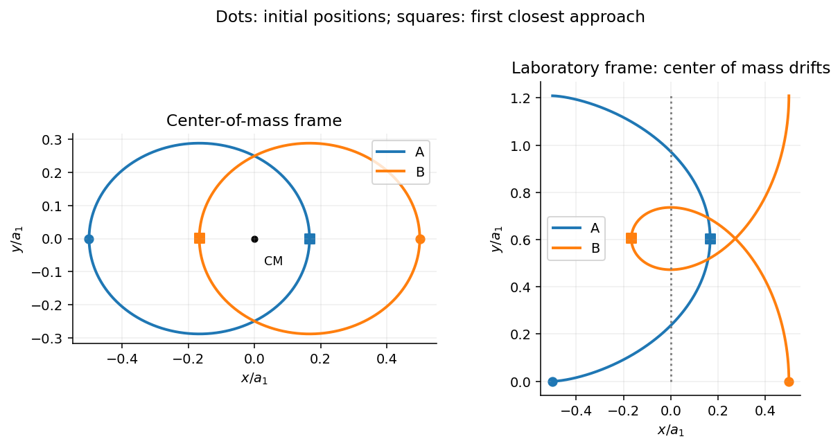
For the two-body problem, define $\mathbf{r}={\mathbf{r}}_B-{\mathbf{r}}_A$, total mass $M=m_A+m_B$, reduced mass $\mu =m_A{m}_B/M$, and center of mass $\mathbf{R}$. The relative equation is $\mu \ddot{\mathbf{r}}=\mathbf{F}$, while the isolated center of mass has $\ddot{\mathbf{R}}=0$. Once the relative orbit is known,The relative energy uses $\mu$ in its kinetic energy and $A=G{m}_A{m}_B$ in the gravitational potential energy.

In the equal-mass case the initial relative speed is $u$, $\mu =m/2$, and the center-of-mass velocity is half B's initial velocity. ThusNegative relative energy requires $u^2<4Gm/a_1$. The escape threshold is $u_E=2\sqrt{Gm/a_1}$; equality is marginal parabolic escape, so a strictly bound pair has $u<u_E$.

For $u=u_E/2=\sqrt{Gm/a_1}$, $E_{\mathrm{rel}}=-3G{m}^2/(4a_1)$ and the relative semimajor axis is $a=2a_1/3$. The initial transverse speed is below the relative circular value $\sqrt{2Gm/a_1}$, so the initial turning point is apoapsis. HenceChoose the initial separation along $+x$ from A to B, with B's initial velocity $+u\hat{\mathbf{y}}$. Conservation of angular momentum gives relative periapsis speed $3u$. At the opposite end of the ellipse the direction is $-\hat{\mathbf{y}}$, soThus B has the same speed as initially but the opposite velocity. A has $2u\hat{\mathbf{y}}$ at that instant. A value $3u/2$ for B would be its center-of-mass-frame speed, not the requested initial laboratory frame result.

The relative orbital period follows from Kepler's third law with total gravitating mass $2m$:In the center-of-mass frame each star follows an ellipse of semimajor axis $a_1/3$ and eccentricity $1/2$, with the center of mass at a focus; they remain opposite on their simultaneous position vectors. In the laboratory frame add the uniform drift $ut/2$ along $y$. The laboratory paths of an equal-mass binary are therefore not closed ellipses, even though their relative motion repeats.

Radial energy and effective potential. For a central force with potential energy $U(r)$, angular momentum conservation fixes $J=m{r}^2\dot{\varphi }$ and confines motion to a plane. The kinetic energy separates into radial and angular parts, givingThe second term is the centrifugal barrier. It converts the radial motion to a one-dimensional energy problem: allowed radii have $E\ge U_{\mathrm{eff}}$, turning points have equality, and a circular orbit occurs at a stationary point of $U_{\mathrm{eff}}$. Stability of that radial orbit requires a local minimum.

The first-order orbit equation. Write $A=GMm$. Since $f=-dU/dr=-A/r^2-A\gamma /r^3$, choose zero potential at infinity to getAlso $\dot{r}=(dr/d\varphi )J/(m{r}^2)$. Substitute this into the energy equation and multiply by $2m{r}^4/J^2$:Here $\gamma$ has units of length. A regular bound orbit with a centrifugal barrier requires $J^2>mA\gamma$ as well as the appropriate negative energy.

Solving in inverse radius. Let $u=1/r$ and defineDividing the first-order equation by $r^4$ givesDifferentiating, or directly using the Binet equation, gives $u^{\prime \prime }+qu=b$. The continuation through turning points follows from this smooth second-order equation. Its noncircular bound solution, with angular origin at a pericentre, isSubstitution into the first-order equation fixes the amplitude through this $e$. Therefore the requested representation holds withsince ${\alpha }_1/r-{\alpha }_2=\cos ({\alpha }_3\varphi )$. A general angular origin replaces $\varphi$ by $\varphi -{\varphi }_0$. This is the orbit equation for combined inverse-square and inverse-cube attraction. The circular limit $e=0$ is regular in $u=b/q$ but is not represented by finite ${\alpha }_1,{\alpha }_2$ in the source's normalized cosine form.

Precession and the inferred length. The last expression immediately givesSuccessive pericentres occur after angular advance $2\pi /{\alpha }_3$, so the apsidal precession per orbit isFor ${\alpha }_3$ near one, $1-{\alpha }_3^2\simeq \Delta \varpi /\pi$. Inferring an inverse-cube perturbation from apsidal precession consequently gives $\gamma \simeq [J^2/(mA)]\Delta \varpi /\pi$. For the stipulated nearly circular approximation, $J^2/(mA)\simeq r_0$, and Kepler's third law givesusing $P=88(86400)\mathrm{s}$, $M=2.0\times 10^{30}\mathrm{kg}$ and $G=6.6743\times 10^{-11}{\mathrm{m}}^3\mathrm{k}{\mathrm{g}}^{-1}{\mathrm{s}}^{-2}$. A century contains about $36525/88=415.1$ orbits. Convert the observed advance to radians per orbit before using it:HenceThe positive sign strengthens the attraction and gives prograde precession. The fractional perturbation $\gamma /r_0\simeq 1.6\times 10^{-7}$ validates the small-deviation expansion. This is the parameter fitting the proposed phenomenological force law under the specified small-eccentricity approximation, not a derivation of that law as the physical explanation of Mercury's anomaly.

A Hohmann transfer orbit connects two coplanar circular orbits using two tangential, effectively instantaneous velocity changes. Take outward transfer radii $r_2>r_1$, and write ${\mu }_g=GM$ for the central body's gravitational parameter. The intervening ellipse has periapsis $r_1$, apoapsis $r_2$, semimajor axis $a_t=(r_1+r_2)/2$ and orbital eccentricity $e=(r_2-r_1)/(r_1+r_2)$.

The circular speed is $\sqrt{{\mu }_g/r}$. Conservation of orbital energy gives the vis-viva equation $v^2={\mu }_g(2/r-1/a_t)$. Therefore the transfer speeds at the two impulses areThe first prograde impulse raises the far side of the orbit; the second prograde impulse raises the near side to circularize at $r_2$. Their magnitudes areThe transfer takes half an ellipse period. Kepler's third law givesFor inward transfer the same ellipse is traversed from apoapsis to periapsis and both burns are retrograde. A rendezvous also needs the correct initial phase of the target: for outward transfer its initial angular lead is $\pi -\sqrt{{\mu }_g/r_2^3}{t}_t$ modulo $2\pi$. The method assumes a two-body gravitational field, negligible atmospheric drag and burns short compared with an orbit. It is an economical two-impulse transfer between these circles; it is not universally the least-$\Delta v$ transfer if additional impulses and very large intermediate radii are permitted.

For two circular Kepler orbits about the same body, Kepler's third law gives $T^2/r^3=\text{constant}$. The reference radius is measured from Earth's centre:A geostationary orbit is prograde and equatorial, with one sidereal day as its orbital period. Using $T_g\simeq 1436\min$ and the supplied $T_1=109\min$,Using $24\mathrm{h}$ instead changes this estimate by less than one per cent. This is the orbital radius, not the altitude; the corresponding altitude is about $3.00\times 10^4\mathrm{km}$.

There is a numerical inconsistency in the source data. The quoted reference orbit implies $G{M}_E=4{\pi }^2{r}_1^3/T_1^2\simeq 2.56\times 10^{14}{\mathrm{m}}^3{\mathrm{s}}^{-2}$, appreciably below the measured terrestrial value, about $3.99\times 10^{14}{\mathrm{m}}^3{\mathrm{s}}^{-2}$. Using the latter instead gives the familiar geostationary orbit radius $4.22\times 10^4\mathrm{km}$. The boxed estimate consistently uses the period actually printed in the question.

For the two-body approximation with a dominant central mass, Kepler's laws of planetary motion are:

The first law includes a circular Kepler orbit as a special case. The third-law constant is the same for bodies orbiting the same dominant mass.

The transfer is a Hohmann transfer orbit. Write $r_0$ for the original circular Kepler orbit radius and $a_t$ for the transfer ellipse's semi-major axis. The diagram measures both radii from Earth's centre, giving $r_1=1.2r_0$, and henceThe Hohmann transfer time is half the transfer orbital period, taking the satellite to the opposite end of the elliptic orbit. By Kepler's third law, relative to the original geostationary orbit's orbital period $T_0$,Using one sidereal day, $T_0=86164\mathrm{s}$, gives $t=4.9703\times 10^4\mathrm{s}=13.806\mathrm{h}$; the usual $24\mathrm{h}$ approximation gives $13.844\mathrm{h}$. The arrival impulse changes the velocity into that of the new circular Kepler orbit without adding coast time in the impulsive model.

There is a real discrepancy between the wording and the diagram: an increase in altitude above Earth's surface is different from the radius increase drawn. If altitude is interpreted literally, let $R_E$ be Earth's radius. Thenusing $R_E\simeq 6371\mathrm{km}$ and $r_0\simeq 42164\mathrm{km}$. Thus $13.8\mathrm{h}$ answers the explicitly labelled geometry; $13.5\mathrm{h}$ answers the literal altitude wording.

For a light test particle of mass $m$ outside a spherical source of mass $M$, Newton's law of universal gravitation gives $\mathbf{F}=-GMm\hat{\mathbf{r}}/r^2$. It is a central force, so its torque about the source vanishes and angular momentum $\mathbf{L}=m\mathbf{r}\times \mathbf{v}$ is conserved. The motion therefore lies in a fixed plane when $L\ne 0$. Its gravitational potential energy is $-GMm/r$, and conservation of mechanical energy givesHere $ϵ$ is specific orbital energy and $h$ is specific angular momentum. A Kepler orbit has polar equationThe angle is measured from periapsis. The conic section is an ellipse for $ϵ<0$ and $0\le e<1$, a parabola for $ϵ=0$ and $e=1$, and a hyperbola for $ϵ>0$ and $e>1$. The circle is the $e=0$ elliptical case. The special case $h=0$ is radial motion and must be handled as a degenerate limit. Bound ellipses have the source at one focus, which is Kepler's first law.

For a bound orbit of semi-major axis $a$, $ϵ=-GM/(2a)$. Combining this with the energy equation gives the vis-viva equation:The particle therefore moves faster near periapsis and slower near apoapsis. Conservation of angular momentum also gives constant areal velocity, $dA/dt=h/2$, expressing Kepler's second law. Using the ellipse's area and $h^2=GMa(1-e^2)$ gives the orbital periodwhich is Kepler's third law.

A circular orbit follows from centripetal acceleration $v_c^2/r=GM/r^2$, giving $v_c=\sqrt{GM/r}$ and $T=2\pi \sqrt{r^3/(GM)}$. The minimum escape velocity from radius $r$ follows from the marginally unbound condition $ϵ=0$:These ideal orbits neglect drag force, other gravitating bodies and changes in the central source. For two comparable masses, the relative two-body problem uses $G(M+m)$ instead of $GM$. An orbiting object is continuously in free fall; the inward gravitational force changes its direction even when its speed is constant. These inverse-square results assume the physical variation of gravity with radius, rather than extending a near-surface constant-$g$ approximation to an entire orbit.

Rearrange the supplied form of Kepler's third law to make the gravitational constant the subject:Convert the semi-major axis and orbital period to SI units before substitution:The central value is thereforeFor monomial uncertainty propagation, logarithmic differentiation givesIf the quoted errors are independent standard uncertainties, the variances of these contributions add:Thus ${\sigma }_G=1.61335\times 10^{-12}{\mathrm{m}}^3\mathrm{k}{\mathrm{g}}^{-1}{\mathrm{s}}^{-2}$, and the measured result under that statistical convention isThe semi-major axis measurement supplies the largest individual contribution to the relative uncertainty.

The paper does not specify whether its errors are statistical uncertainties or bounds. If they are maximum input errors, the first-order worst-case error propagation estimate adds magnitudes:Correlation between input errors would instead require the covariance terms in the general propagation of uncertainty formula; they are not specified.

Write $A(r)=1-2\mu /r$, with $\mu =GM/c^2$. On the equatorial plane, the geodesic Lagrangian isThe coordinates $t$ and $\varphi$ are cyclic, giving $\boxed{A\dot{t}=k,r^2\dot{\varphi }=h}$. The conserved physical energy per unit rest mass is $c^{2}k$, while $h$ is the signed angular momentum per unit rest mass. The radial Euler-Lagrange equation, with $A^{\prime }=2\mu /r^2$, isThese are the requested geodesic equations. The equatorial condition is consistent with the polar equation by the spherical symmetry of the Schwarzschild metric.

The normalization of the four-velocity is $c^2=c^{2}A{\dot{t}}^2-A^{-1}{\dot{r}}^2-r^2{\dot{\varphi }}^2$. Insert the two conserved quantities and multiply by $A$ to obtainThis is a one-dimensional radial energy equation. Half of its left side is radial kinetic energy per unit mass plus an effective potential: the Newtonian centrifugal and gravitational terms acquire the extra attractive contribution $-\mu h^2/r^3$.

A timelike circular Schwarzschild geodesic requires $\dot{r}=\ddot{r}=0$. Equivalently, set the derivative of $V(r)=h^2/r^2-2\mu h^2/r^3-2\mu c^2/r$ to zero. At $r=R$ this gives $h^2(R-3\mu )=\mu c^2{R}^2$, and substitution in the radial energy equation yieldsSuch timelike circular orbits require $R>3\mu$. Their coordinate angular velocity satisfies ${\Omega }^2=\mu c^2/R^3$, and their proper clock rate is $d{\tau }_s/dt=A/k=\sqrt{1-3\mu /R_s}$.

For the static North-Pole clock, $d{\tau }_E/dt=\sqrt{1-2\mu /R_E}$. Consecutive overhead passages occur one coordinate orbital period apart, and the repeated Earth-satellite geometry gives equal signal travel delays. The comparison of circular-orbit and static Schwarzschild clocks therefore givesThis includes both gravitational and orbital-motion effects; a separate Newtonian time-dilation correction must not be added again.

For an estimate, Kepler's third law gives $R_s=42100\mathrm{km}(3/24{)}^{2/3}=10525\mathrm{km}$. The same approximate geostationary radius and period give $\mu =4{\pi }^2{R}_{\mathrm{geo}}^3/(c^2{T}_{\mathrm{geo}}^2)\simeq 4.4\mathrm{mm}$. Expanding the ratio to first order,The satellite clock consequently gains about $0.7\mu \mathrm{s}$ over a three-hour orbit in this approximation. The surface observer is taken to be static, and the spacetime model is the spherical Schwarzschild metric specified in the problem.

Kepler's third law for two point masses in a Newtonian gravitational field isHere $a$ is the semimajor axis of their relative orbit, $P$ the orbital period and $G$ the gravitational constant. Equivalently $(P/\mathrm{yr}{)}^2=(a/\mathrm{AU}{)}^3/[(M_1+M_2)/M_{\odot }]$, to the accuracy with which these astronomical units normalize the solar mass.

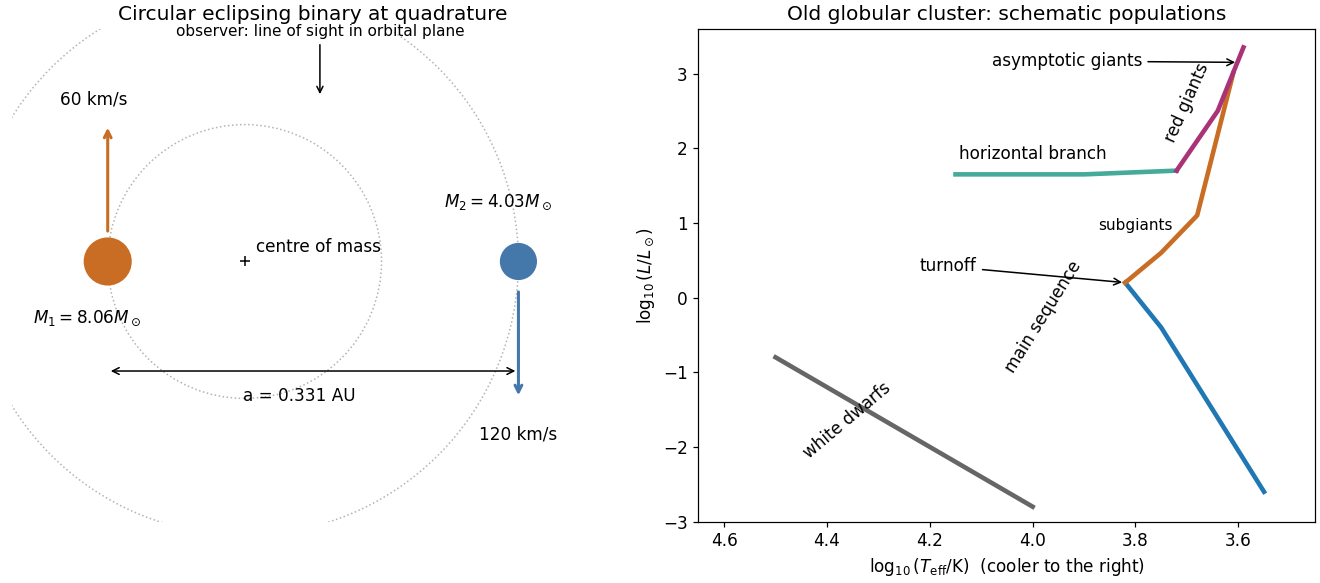
Assume a circular orbit and an orbital inclination $i\simeq 90^{\circ }$, as appropriate for a simple eclipsing binary estimate. At quadrature the two radial velocities are opposite and equal to the orbital speeds. The more massive component has the smaller amplitude. With the centre of mass as origin,Thus $a_1=0.1103\mathrm{AU}$, $a_2=0.2206\mathrm{AU}$ and Kepler's third law givesThe orbital plane contains the observer's line of sight; at quadrature the two velocities point towards and away from that observer, as labelled in the original schematic below. For an elliptic orbit, the measured amplitudes instead give $a\sin i=P(K_1+K_2)\sqrt{1-e^2}/(2\pi )$; the numerical answer requires the circular assumption.

The intact source figure gives orbital period $P=6.0\mathrm{yr}$, stellar radial velocity semiamplitude $K=30.0\mathrm{m}{\mathrm{s}}^{-1}$, and orbital eccentricity $e=0$. A planetary exoplanet transit implies a nearly edge-on orbit, so $\sin i\simeq 1$. Adopt a solar mass for the Solar-type star and initially neglect the companion's mass relative to it.

For a circular solution of the two-body problem, the star's distance from the centre of mass is $a_{\ast }=a{M}_p/(M_{\ast }+M_p)$, and the measured semiamplitude is $K=2\pi a_{\ast }\sin i/P$. Kepler's third law givesHenceThe inferred binary mass ratio is only $0.00183$, validating the approximation. Since $e=0$, the star–planet separation is constant and equals the orbital semimajor axis. Without the exoplanet transit, Doppler spectroscopy would generally give only a minimum companion mass through $M_p\sin i$.

Doubt was reasonable if it concerned the physical cause or unlimited extrapolation of Newton's law of universal gravitation; wholesale dismissal of the quantitative evidence was harder to justify. Early eighteenth-century investigators had to distinguish the success of an inverse-square force law in explaining observations from the claim that every material body directly attracts every other one without a mediating mechanism.

The strongest case for Isaac Newton's framework was its unification of phenomena previously treated separately. Kepler's third law and nearly elliptic orbits could be connected to an inverse-square central force. Comparing terrestrial gravity with the centripetal acceleration of the Moon supported continuity between falling bodies and celestial motion. The Philosophiae Naturalis Principia Mathematica by Isaac Newton also developed treatments of interacting bodies, tides and the Earth's figure. These were substantive tests and organized a research programme capable of producing further quantitative comparisons.^[ref]

There were nevertheless rational reservations. A law proportional to $m_1{m}_2/r^2$ inferred from accessible bodies and distances did not logically establish unrestricted universality. Individual celestial predictions involved uncertain observations and approximations to difficult many-body classical mechanics. The Moon's motion and the Earth's shape were demanding tests whose successful treatment was not complete at the beginning of the century. A dissenter could question auxiliary assumptions, numerical accuracy or the inference from special cases without denying every success.

A deeper objection concerned explanation. In traditions requiring contact mechanisms, unexplained attraction across empty space appeared to reintroduce an occult quality. René Descartes's vortices supplied a mechanical alternative, though they faced their own serious dynamical difficulties. Newton himself separated a mathematically established pattern from a claimed cause of gravity; the 1713 General Scholium by Isaac Newton declined to invent an unsupported physical mechanism. Treating every criticism of action at a distance as a failure to understand evidence would therefore misrepresent the available positions.^[ref]

Later confirmations cannot be counted as evidence already possessed by an early-eighteenth-century critic. Subsequent geodetic measurements, improved lunar theory and successful comet predictions helped shift the balance, but their timing matters. Nor did retaining a mechanical alternative remain equally reasonable after every failed prediction: responsible doubt required comparative assessment and willingness to revise it. The balanced conclusion is that selective, explicit scepticism about universality or cause was defensible, while the breadth of Newtonian mechanics' quantitative achievements already imposed a substantial explanatory burden on rival accounts.

Kepler's third law for two point masses in a Newtonian gravitational field isHere $a$ is the semimajor axis of their relative orbit, $P$ the orbital period and $G$ the gravitational constant. Equivalently $(P/\mathrm{yr}{)}^2=(a/\mathrm{AU}{)}^3/[(M_1+M_2)/M_{\odot }]$, to the accuracy with which these astronomical units normalize the solar mass.

Assume a circular orbit and an orbital inclination $i\simeq 90^{\circ }$, as appropriate for a simple eclipsing binary estimate. At quadrature the two radial velocities are opposite and equal to the orbital speeds. The more massive component has the smaller amplitude. With the centre of mass as origin,Thus $a_1=0.1103\mathrm{AU}$, $a_2=0.2206\mathrm{AU}$ and Kepler's third law givesThe orbital plane contains the observer's line of sight; at quadrature the two velocities point towards and away from that observer, as labelled in the original schematic below. For an elliptic orbit, the measured amplitudes instead give $a\sin i=P(K_1+K_2)\sqrt{1-e^2}/(2\pi )$; the numerical answer requires the circular assumption.

The common one-per-cent exoplanet transit depth gives $R_p=0.1R_{\star }$. Apply the supplied main-sequence mass-radius relation, $R_{\star }/R_{\odot }=M_{\star }/M_{\odot }$, and Kepler's third law, neglecting the planet mass. For $P=6$ days,The companions are approximately Jupiter-sized and Earth-sized respectively; these are sizes, not independently determined masses. The duration uses the small-planet chord approximation. Counting the finite planet radius would increase first-to-fourth-contact durations by about ten per cent for central transits.

For equal distance, passband, cadence and noise dominated by stellar photon counting, the supplied mass-luminosity relation makes the solar-mass host about $10^3$ times more luminous, with a transit about $4.64$ times longer. At equal fractional exoplanet transit depth, signal-to-noise per event scales as $\delta \sqrt{{\dot{N}}_{\gamma }{t}_{\mathrm{tr}}}$, favouring the solar-mass host by about $\sqrt{1000\times 4.64}\simeq 68$. Equal apparent brightness would remove the luminosity advantage but retain the duration advantage. Without distances and noise properties the relative detectability is conditional. Transit probability is also larger for the solar-mass case, about $7.2\%$ versus $1.55\%$.

The habitable zone is the range of orbital distances where an appropriate planetary atmosphere could sustain liquid water at the surface; it is not a guarantee of inhabited or even habitable conditions for every planet. At a fixed habitable incident flux, $a_{\mathrm{HZ}}\propto L_{\star }^{1/2}$. With the supplied $L_{\star }\propto M_{\star }^3$, Kepler's third law givesTaking Earth as a rough central reference, a $0.1M_{\odot }$ star has $a_{\mathrm{HZ}}\sim 0.0316\mathrm{AU}$ and $P_{\mathrm{HZ}}\sim 6.5$ days. Its six-day, Earth-sized companion receives about $1.11$ times terrestrial irradiance and could therefore lie in the habitable zone in this simplified model. Atmosphere, stellar activity, tidal locking and volatile retention remain unknown. The six-day companion around the Sun-like star receives about $239$ times terrestrial irradiance and is approximately Jupiter-sized; it is not a plausible surface-water Earth analogue. The stellar spectral dependence of actual habitable-zone edges is omitted by the simple scaling.