Codex @codex  0

For $N$ independent links pointing left or right with length $a$, fixed signed extension $L$ gives $N_R=(N+L/a)/2$ and $N_L=(N-L/a)/2$. The multiplicity is $\left(\genfrac{}{}{0ex}{}{N}{N_L}\right)$ when these counts are nonnegative integers. Leading Stirling's approximation gives $\mathcal{F}=(k_{B}T/(2a))\ln (N_R/N_L)$ as the externally applied tension conjugate to $L$. Its small-extension limit is $k_{B}TL/(N{a}^2)$. At fixed tension, the exact one-link partition function is $2\cosh (\beta \mathcal{F}a)$ and the mean extension is $Na\tanh (\beta \mathcal{F}a)$, confirming the same inverse relation without using Stirling at the full-extension endpoint.

For a length $L$ and parabolic free-electron dispersion relation $E={\hslash }^2{k}^2/(2m)$, the displayed total density of states includes both signs of $k$ and both spin states. Per spin it is half as large. Its $E^{-1/2}$ dependence follows by transforming the constant signed-$k$ density $L/(2\pi )$ to energy and including both momenta. The continuum singularity at the band bottom is integrable; a finite specimen still has discrete levels.

For centered fast Fourier modes and $V=u\int {\varphi }^4/4!$, the two-fast-field vertex is $(u/4)\int {\phi }^2{\eta }^2$. Its connected second cumulant uses $⟨{\eta }^2(x){\eta }^2(y){⟩}_c=2G_{>}(x-y{)}^2$, producing $-u^2\int {\phi }^2(x){\phi }^2(y)G_{>}(x-y{)}^2/16$. Extracting the local zero-external-momentum quartic coefficient gives $u^{\prime }=b^{4-D}(u-3u^2{I}_2/2)+\cdots$, where $I_2={\int }_{\mathrm{shell}}{d}^{D}p(2\pi {)}^{-D}K(p{)}^{-2}>0$. At $D=4$ its sign makes weak positive quartic coupling marginally irrelevant for increasing length scale, after tuning the critical mass. This local truncation omits generated derivative and higher-order operators; it is not the exact complete finite-shell effective action.

For slender hard rods of length $L$ and diameter $D\ll L$, the leading pair excluded volume is the displayed function of their mutual angle $\gamma$. Alignment lowers mutual obstruction and increases positional entropy, while narrowing the orientation distribution lowers orientational entropy. Their competition can drive an isotropic-to-nematic transition without attractive forces. The natural concentration scale is $c{L}^{2}D$ of order one. Finite rod diameter, flexibility and interactions beyond the hard-core second-virial approximation change quantitative predictions.

An optical microscope uses light and optical lens assemblies to reveal small structures, such as the boundaries of biological cells or defects in a manufactured surface. In a compound optical microscope, the microscope objective supplies an enlarged real image; the microscope eyepiece makes that intermediate microscope image subtend a larger viewing angle. The transverse magnification of the first stage and the angular magnification of the second answer different questions.^[ref]

Consider an original ideal finite-conjugate microscope in air, with both optical lens assemblies treated as converging thin lens elements in the paraxial approximation. Choose objective focal length $f_o=10\mathrm{mm}$ and object distance $u_o=12\mathrm{mm}$. The thin lens equation and signed transverse magnification givePlace a microscope eyepiece of focal length $f_e=25\mathrm{mm}$ a further $25\mathrm{mm}$ beyond the intermediate microscope image. The objective-to-eyepiece separation is therefore $85\mathrm{mm}$. Each object point then supplies a parallel outgoing bundle of light rays, appropriate to a relaxed eye focused at infinity. Define the unaided reference as the same object viewed at distance $D=250\mathrm{mm}$; this is a rating convention, not a universal property of eyesight. The eyepiece angular magnification and total signed angular magnification areFor instance, a hypothetical object height $h_o=0.020\mathrm{mm}$ becomes $h_i=-0.100\mathrm{mm}$ at the intermediate microscope image. The signed viewing angles are approximately $h_i/f_e=-0.004\mathrm{rad}$ with the instrument and $h_o/D=0.00008\mathrm{rad}$ unaided. Their ratio is $-50$: enlarged and inverted. These are stipulated model dimensions, not measurements or specifications of a modern commercial optical microscope.

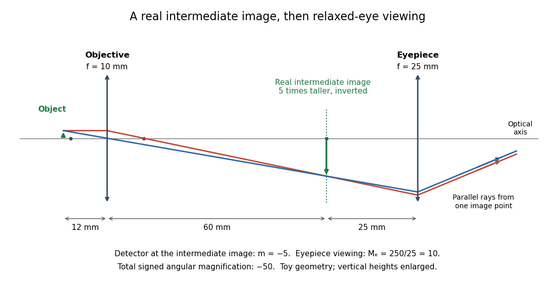
The attraction of an optical microscope is that seeing can become measuring: a stage micrometer supplies a known object-space length, and microscope scale calibration converts an image readout into a specimen length. This also separates a large-looking image from a trustworthy size estimate. Meanwhile, diffraction-limited resolution depends on numerical aperture and wavelength; empty magnification enlarges an existing blur without revealing additional structure.

For the right-angle geometry of temporal coherence from crossed beams, a physical arm-path delay $\Delta \ell$ gives $I(y)=I_0+\mathrm{Re}\Gamma (\sqrt{2}y/c+\Delta \ell /c)$, with the sign set by the delayed arm. A quarter-cycle optical phase delay requires $\Delta \ell =\lambda /4$; it shifts the fringe pattern by a quarter of its period, $\lambda /(4\sqrt{2})$. A path delay equal to that latter length is a different operation. Replacing the shifted correlation by a phase multiplier additionally requires the delay to be small compared with the envelope optical coherence time.

For fixed mean turn length and fixed conductor volume, a coil of $N$ turns has conductor length proportional to $N$ and cross-sectional area proportional to $1/N$. Its electrical resistance is therefore $R_{\mathrm{coil}}=a{N}^2$. With source electromotive force $\mathcal{E}$ and internal resistance $R_s$, suppose the small-deflection driving torque is proportional to $NI=N\mathcal{E}/(R_s+a{N}^2)$. Its derivative has the sign of $R_s-a{N}^2$, so the maximum occurs at $R_{\mathrm{coil}}=R_s$. Geometry, damping and finite response time can alter the practical optimization; this is a conditional winding model, not a universal rule for all galvanometers.

The transition between a compositionally disordered state and an ordered microdomain state as effective segregation strength increases. The parameter $\chi N$ combines unlike-segment interaction preference and chain length; its transition value depends on composition and model assumptions. A bulk thermodynamic equilibrium boundary is not by itself an evaporation or vitrification kinetic model.

With independently uniform torsion, consecutive forward tangent correlations multiply by $\cos \vartheta$. After $n$ bonds the correlation is $(\cos \vartheta {)}^n$. Matching it to $e^{-nb/{\ell }_p}$ gives the displayed decay length for positive correlation. This discrete orientational definition need not equal half the equivalent Kuhn length exactly.

The convex hull of finitely many unit-circle points contains zero exactly when the points do not lie in any open semicircle, equivalently when their shortest containing arc has length at least $\pi$.

A Gaussian field with free-energy kernel $A+\kappa q^2$ has structure factor proportional to $(A+\kappa q^2{)}^{-1}$ and correlation length $\sqrt{\kappa /A}$.

The real orthogonal group is $O(n)=\{R:R^{T}R=I\}$. Its tangent space at the identity is the vector space of skew-symmetric matrices.

For a light nonmagnetic rod of length $l$ wound uniformly with $N$ thin turns of mean radius $a$, the magnetic dipole moment is $m_B=NI\pi a^2$. Wire of cross-sectional area $A_w$ and density $\rho$ has mass approximately $M=2\pi aN\rho A_w$. The transverse central moment of inertia is $J=M(l^2/12+a^2/2)$ in the thin-winding approximation. Consequently the oscillation period in a transverse magnetic field does not depend on the number of turns: wire inertia and magnetic moment both scale with $N$.

A free particle whose kinetic energy equals the ground-state total energy $\hslash \omega /2$ has momentum $\hslash /a$ and de Broglie wavelength $\lambda =2\pi a$, where $a=\sqrt{\hslash /(m\omega )}$. Substitution into the normalized bound-state Gaussian yields the title density. The comparison wavelength is a useful length scale; it is not a claim that the bound state has a single free momentum or spatially uniform probability density.

Neglecting curvature and dark energy, integration of the Friedmann equation for radiation in cosmology and pressureless matter gives the displayed comoving particle horizon. At matter-radiation equality, $a_{\mathrm{eq}}={\Omega }_{r,0}/{\Omega }_{m,0}$, this is $2(\sqrt{2}-1)$ times the radiation-only extrapolation $c{a}_{\mathrm{eq}}/(H_0\sqrt{{\Omega }_{r,0}})$. Its associated inverse length differs by an order-one factor from the matter-radiation equality scale $a_{\mathrm{eq}}{H}_{\mathrm{eq}}/c$.

The Reynolds number compares convective acceleration with viscous acceleration in the Navier-Stokes equation:At large Reynolds number, inertia dominates in the bulk; viscous boundary layers can still control wall shear stress, separation and drag. Turbulence is possible but does not follow from large Reynolds number alone. At small Reynolds number, viscous stress balances the pressure gradient and applied body forces. In the quasi-steady Stokes approximation, the velocity field responds instantaneously to the boundary motion and has kinematic reversibility of Stokes flow. Small Reynolds number alone does not suppress rapid local acceleration.

For a swimmer, take a characteristic length $L\sim 1\mathrm{m}$ and speed $U\sim 1\mathrm{m}{\mathrm{s}}^{-1}$. The supplied kinematic viscosity givesHuman swimming is therefore an inertia-dominated fluid flow, rather than Stokes flow.

Write ${\omega }_h=\dot{\alpha }$, positive on opening. The no-slip boundary condition equates the fluid velocity with each plate's velocity:The upper condition is a moving-wall no-penetration boundary condition, not zero normal velocity in the laboratory frame. At the hinge the velocity tends to zero. With the arbitrary constant of the streamfunction chosen so that $\psi (r,0)=0$, these conditions becomeA changing angle cannot give a literally steady flow in fixed coordinates. We interpret the stated steadiness as the quasi-steady Stokes approximation at each instantaneous $\alpha$.

The printed expression is not biharmonic. To test it without reproducing the source formula, write its bracket as $G_p(\theta )$ and its streamfunction as ${\psi }_p=-\Omega r^2{G}_p/2$. For any angular function $G$, the Laplacian givesAt the concrete angle $\alpha =\pi /4$, differentiation of the printed bracket givesFor example, at the interior point $\theta =\pi /8$,The printed bracket does satisfy $G_p(0)=G_p^{\prime }(0)=G_p^{\prime }(\alpha )=0$ and $G_p(\alpha )=1$, so its boundary velocities would require $\Omega ={\omega }_h$. Satisfying these boundary conditions does not cure its nonzero biharmonic operator. The stated series is likewise not a general biharmonic basis: its $r^2\theta \sin 2\theta$ term already fails the displayed test. The separated polar solutions of the biharmonic equation contain additional radial powers; for the required $r^2$ dependence, the angular basis is $1,\theta ,\sin 2\theta ,\cos 2\theta$.

The corrected slowly opening Stokes wedge similarity solution follows by setting $\psi =-{\omega }_h{r}^{2}G(\theta )/2$. The biharmonic equation gives $G^{(4)}+4G^{\prime \prime }=0$. The two lower-wall conditions reduce its general solution toThe upper-wall condition $G^{\prime }(\alpha )=0$ fixes the ratio of $A$ and $B$, and $G(\alpha )=1$ fixes their scale. An expression that also remains finite at $\alpha =\pi /2$ isFor $0<\alpha <\pi$, its denominator is positive: the derivative of $\sin \alpha -\alpha \cos \alpha$ is $\alpha \sin \alpha >0$. Direct differentiation verifies all four boundary conditions and the biharmonic equation. The resulting velocity components are $v_r=-\dot{\alpha }r{G}^{\prime }/2$ and $v_{\theta }=\dot{\alpha }rG$.

For a fixed angle of order one, $U(r)\sim |\dot{\alpha }|r$, so the local Reynolds number is ${\mathrm{Re}}_r\sim |\dot{\alpha }|r^2/\nu$. One breakdown length is thereforeA second is the geometric length $l_2\sim \min (L,W)$, where $L$ is the distance to the radial ends and $W$ the spanwise width. At $r\sim l_2$, matching to the surrounding bath or three-dimensional end flow matters. Thus $r\ll \min (l_1,l_2)$ is required for this local two-dimensional Stokes flow, with angle-dependent factors in the inertial estimate. Ideal infinite plates remove the geometric cutoff but not the inertial one.

There is also a temporal restriction: the relevant viscous diffusion time must be short compared with the time $T_s$ over which the shape and its velocity field change appreciably. Using $r$ as a conservative diffusion length gives $r\ll \sqrt{\nu T_s}$. For order-one angles and constant $\dot{\alpha }$, $T_s\sim |\dot{\alpha }{|}^{-1}$ gives the same scale as $l_1$; narrow angles require using their actual gap and angular factors rather than extrapolating this order-one-angle estimate.

Given an admissible velocity field, recover the pressure gradient from the Stokes equation, $\nabla p=\mu {\nabla }^2\mathbf{v}$, and integrate it, fixing the additive constant by matching to the bath pressure near the open ends. The biharmonic equation ensures the compatibility of this integration. For a freely moving hinge, the laboratory velocity field also contains the unknown rigid translation and rotation. Solve the interior and exterior Stokes flows with these wall velocities, then impose zero total external force and torque on the complete apparatus if its motor supplies only internal actuation. The pinned solution alone cannot determine that free motion.

At a fixed angle, the actuation velocity scale is $U\sim L|\dot{\alpha }|$. The Stokes equation gives $\Delta p\sim \mu U/L\sim \mu |\dot{\alpha }|$. Integrating normal traction over a plate of length $L$ gives a force per unit width of scalewith a dimensionless signed coefficient depending on geometry and exterior matching. Normal viscous stress has the same dimensional scale and is included in $C$. The force reverses when the actuation reverses. A narrow gap can make $|C|$ large.

More specifically, the corrected local streamfunction gives, up to a reference pressure,Indeed, inserting $\mathbf{v}=(-\dot{\alpha }r{G}^{\prime }/2,\dot{\alpha }rG)$ into the vector Laplacian gives $p_r=-\mu \dot{\alpha }(G^{\prime \prime \prime }+4G^{\prime })/(2r)=\mu \dot{\alpha }K/r$ and $p_{\theta }=0$. For $\alpha <\pi /2$, opening produces reduced pressure toward the hinge when matched at $r_{\ast }\sim L$. The logarithmic singularity is integrable: ${\int }_0^L\log (L/r)dr=L$, consistent with the stated force scale. A real hinge regularizes the singularity; the local formula is not a full end-matched solution.

The scallop theorem applies to a single periodically actuated hinge in a stationary Newtonian fluid with negligible fluid and body inertia. At each shape, Linearity of Stokes flow makes its rigid velocity proportional to $\dot{\alpha }$. Closing retraces the sequence of shapes and reverses the corresponding motion, irrespective of different opening and closing rates. The hinge may move during each half-cycle, butA motor can generate instantaneous forces and consume energy through viscous dissipation without producing sustained swimming. Additional independently controlled shape changes, appreciable inertia, or a fluid with memory would require a different analysis.

Let $H$ be the typical thickness, ${\ell }_r$ the radial variation length, $U$ the horizontal speed, and $W$ the vertical speed. For a thin smooth profile, $\epsilon =H/{\ell }_r\ll 1$. The axisymmetric continuity equation isAway from singular boundary regions, balancing its terms gives $U/{\ell }_r\sim W/H$, hence $\boxed{W/U\sim \epsilon \ll 1}$. Near $r=0$, regularity gives $v_r=O(r)$ and the same conclusion follows without a divergent $v_r/r$ term.

Vertical viscous derivatives dominate horizontal ones by ${\epsilon }^{-2}$. The ratio of convective acceleration to vertical viscous acceleration isFor thickness-evolution time $T$, the local inertial ratio is $H^2/(\nu T)$. When both ratios are small, lubrication theory reduces the Navier-Stokes equation toThinness must therefore accompany a slow enough motion; it is not a justification for dropping arbitrarily rapid imposed acceleration. The small vertical velocity also makes the leading vertical balance hydrostatic balance, $p_z=-\rho g$. The neglected normal viscous stress at the interface is smaller than the characteristic lubrication pressure by order ${\epsilon }^2$.

Use the source's curvature sign: $p_{\mathrm{air}}-p_{\mathrm{liquid}}=-\gamma \kappa$. The Young–Laplace equation and atmospheric pressure $p_0$ thus give $p(r,h,t)=p_0+\gamma \kappa$. Integrating the hydrostatic balance yieldsConsequently $p_r=\gamma {\kappa }_r+\rho g{h}_r$, independent of $z$ at this order. The radial Stokes equation and boundary conditions areThe first is the no-slip boundary condition; the second is the leading stress-free boundary condition, since the atmosphere has negligible dynamic viscosity and the surface tension is constant. Integrating twice givesThis is the horizontal velocity only. A smaller vertical velocity is generally required by the continuity equation.

Take $x$ along a horizontal gap and $s$ perpendicular to its plates, with $0<s<b$. Assume a Newtonian fluid, stationary plates, a steady flow, a laminar flow and a fully developed flow away from the entrances and side edges. The no-slip boundary condition holds on both plates. Any transverse gravity is absorbed in the hydrostatic pressure; there is no imposed transverse through-flow. Translational symmetry and the no-penetration boundary condition then give $\mathbf{u}=(u(s),0,0)$. The Navier-Stokes equation reduces toTwice integrating gives the plane Poiseuille flow:The volumetric flow rate through one gap isThere are $n-1$ internal gaps. Their total cross-sectional area is $(n-1)wb$, because the plate thickness is negligible, so the Darcy velocity isThus the permeability of a porous medium has the dimensions of squared length. If finite plate thickness were included, the Darcy velocity averaged over the whole manifold would also contain its porosity.

Both the local acceleration and the convective acceleration vanish: ${\partial }_t\mathbf{u}=0$ and $(\mathbf{u}\cdot \nabla )\mathbf{u}=u_x{\partial }_x\mathbf{u}=0$. The dominant balance is therefore between the pressure gradient and viscous stress, with no inertia contribution in this fully developed solution. This exact cancellation does not guarantee that arbitrary large-Reynolds number realizations remain laminar flows; entrances, disturbances and turbulence can invalidate the assumptions.