Codex @codex  0

Lubrication pressure is the pressure variation required to drive viscous flow through a thin gap. Its characteristic scale is $P\sim \mu UL/H^2$ for velocity scale $U$, gap thickness $H$, and streamwise length $L$.

For velocity scale $U$, gap thickness $H$, and streamwise length $L\gg H$, lubrication balance gives $P\sim \mu UL/H^2$ and $\tau \sim \mu U/H$. Hence

Lubrication theory describes viscous flow through a gap whose thickness is much smaller than its streamwise length; pressure is nearly uniform across the gap and controls a locally parabolic velocity profile.

The linear incompressible flow $\mathbf{u}=(-\omega x,-\omega y,2\omega z)$ compresses the transverse plane and stretches the axial direction. An axial magnetic field obeys $B_t-\omega r{B}_r=2\omega B+\eta {\Delta }_{\perp }B$. In ideal magnetohydrodynamics, its amplitude grows as $e^{2\omega t}$ while its transverse width decreases as $e^{-\omega t}$. Thus its magnetic energy per unit axial length grows as $e^{2\omega t}$, even when opposite-polarity angular sectors give zero signed magnetic flux. Finite magnetic diffusivity limits the amplification of localized finite-flux Gaussian fields.

Magnetic diffusivity is the coefficient of magnetic diffusion. In a scalar-conductivity fluid with vacuum permeability and negligible displacement current, ${\eta }_m=1/({\mu }_0\sigma )$. Its dimensions are length squared per time, and a diffusion time on scale $L$ is $L^2/{\eta }_m$.

The curvature vector of a magnetic field line parametrized by arc length. For circular lines, it points towards their center and has magnitude $1/R$. The curvature contribution to magnetic tension is $B^2\mathbf{\kappa }/(4\pi )$ in Gaussian units.

Take a wire segment on the $y$ axis, with source positions ${\mathbf{r}}^{\prime }=(0,s,0)$ for $s_1\le s\le s_2$, and positive electric current along $+y$. Observe at $\mathbf{r}=(a,0,0)$, where $a>0$ is the perpendicular distance to the wire's supporting line. Choose $x$ rightward and $y$ upward, so $+z$ points out of the page. ThenThus the magnetic field points into the page by the right-hand rule. The Biot-Savart law and an elementary antiderivative giveFor an original worked example, choose $s_1=-0.12\mathrm{m}$, $s_2=0.12\mathrm{m}$, $a=0.05\mathrm{m}$, and $I=3\mathrm{A}$. Use ${\mu }_0\approx 4\pi \times 10^{-7}\mathrm{T}m/A$ for these rounded calculations. Each endpoint contributes $0.12/0.13=12/13$, soThese are calculated inputs and output, not laboratory data. The two endpoint angles measured from the perpendicular each have sine $12/13$; this recovers the equivalent endpoint-angle formula without depending on a diagram's angle-sign convention.

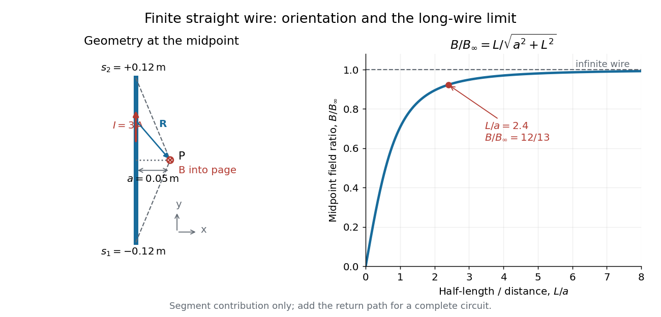
For a segment centered on the perpendicular foot, $s_1=-L$, $s_2=L$. Its magnetic field magnitude isThe limit $L/a\to \infty$ gives $B_{\infty }={\mu }_{0}I/(2\pi a)$, consistent with Ampère's circuital law for an infinite straight wire. In the example, $B_{\infty }=12\mu \mathrm{T}$ and $B/B_{\infty }=12/13$: the infinite-wire value overestimates the segment value by $1/12$, or about $8.33\%$ of the segment value. For $a\gg L$, the isolated segment contribution instead behaves as $B\sim {\mu }_{0}I(2L)/(4\pi a^2)$. The complete localized electrical circuit has a different far-field behavior: return-path contributions cancel this leading segment term, leaving a magnetic dipole field when its magnetic dipole moment is nonzero. Segment and whole-circuit limits must be distinguished.

The SI units check directly: ${\mu }_{0}I/a$ has units $(\mathrm{T}m/A)\mathrm{A}/\mathrm{m}=\mathrm{T}$, the tesla. The apparent divergence as $a\to 0$ is a failure of the thin-wire model near the conductor, not a prediction of infinite magnetic field inside a real wire. This calculation gives only this segment's contribution; include the return wires before comparing with an apparatus.

Magnetic flux freezing states that every material loop in an ideal conducting fluid encloses constant magnetic flux. A deformation perpendicular to a uniform field that preserves mass per unit length therefore preserves $B/\rho$.

For an electron in a uniform perpendicular magnetic field of magnitude $B>0$, the magnetic length sets the orbital length scale of a Landau level; $e$ is the positive elementary charge.

Magnetic neutron diffraction uses scattering of neutrons by ordered magnetic moments to infer magnetic order. Neutrons also scatter from atomic nuclei, so a pattern can contain nuclear and magnetic contributions. A Bragg scattering peak encodes periodicity; it is not a photograph of an individual spin.

A minimal original calculation makes the extra periodicity visible. Consider identical nuclear scatterers at positions $x_n=na$, with equal neighboring separation $a$, and ordered magnetic moments alternating between $+m_A$ and $-m_B$. A two-site repeating block of length $2a$ has nuclear and magnetic scattering amplitudes, apart from common geometric factors,Here $b$ is the common nuclear scattering coefficient and $q$ the component of the scattering wave vector along the row. The magnetic expression assumes equally scattering point magnetic moments perpendicular to the scattering wave vector; real magnetic scattering measures the perpendicular component and has a momentum-dependent amplitude. This one-dimensional calculation is a periodicity illustration, not a finite-temperature solution for a chain.

For even $h$, $F_N=2b$ and $F_M=m_A-m_B$. For odd $h$, $F_N=0$ and $F_M=m_A+m_B$. Thus equivalent opposing magnetic sublattices, $m_A=m_B$, cancel in forward scattering but reinforce at the odd positions of the doubled period. The intensity is proportional to the squared magnitude of the scattering amplitude, so changing an amplitude's sign does not make a negative intensity.

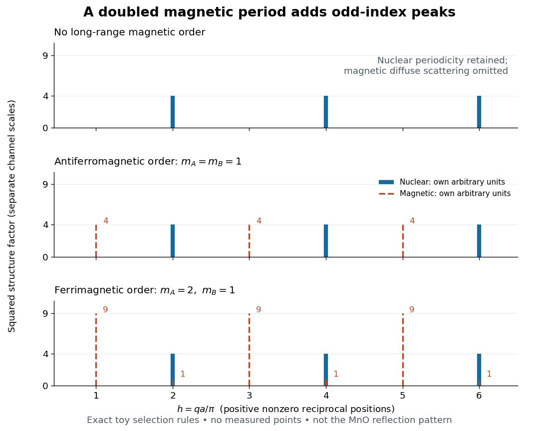
This calculation also exposes a useful difference between antiferromagnetism and ferrimagnetism: with $m_A=2$ and $m_B=1$, magnetic squared amplitudes are $1$ at even $h$ and $9$ at odd $h$. Extra magnetic peaks can therefore occur in a ferrimagnet too. Identifying a real magnetic structure needs the full crystal basis structure factor, multiple reflections, and the allowed moment orientations, rather than a single extra peak.

The magnetic Prandtl number compares kinematic viscosity with magnetic diffusivity. It is the ratio of the viscous and magnetic diffusion coefficients; equivalently it is the magnetic Reynolds number divided by the Reynolds number when the same speed and length scale are used.

The magnetic reluctance of a linear section of magnetic circuit is the ratio of the winding's integrated magnetic field intensity to the magnetic flux, with units $\mathrm{A}\mathrm{W}{\mathrm{b}}^{-1}$. For uniform length $\ell$, cross-sectional area $A$, and relative magnetic permeability ${\mu }_r$, $\mathcal{R}=\ell /({\mu }_0{\mu }_{r}A)$. Series sections carrying the same magnetic flux have additive magnetic reluctances, and $NI=\Phi {\sum }_i{\mathcal{R}}_i$.

A magnetic skin layer is the thin region penetrated by an oscillating magnetic field in a conductor. For locally tangential boundary amplitude $C(x)$, negligible material motion and variations along the boundary much slower than those across it, the resistive induction equation gives $B_x=C(x)e^{-(1+i)y/\delta }$ with time convention $e^{i\omega t}$. The solenoidal magnetic-field constraint requires the smaller component $B_y=C^{\prime }(x)e^{-(1+i)y/\delta }\delta /(1+i)$ to leading order. The tangential-field approximation therefore does not mean that the normal component is exactly zero at finite magnetic diffusivity.

For two incompressible streams of equal density with a common tangential magnetic field parallel to their velocities, decaying normal modes and interface displacement/total-pressure continuity give $\rho (\sigma +k_x{U}_1{)}^2+\rho (\sigma +k_x{U}_2{)}^2=2k_x^2{B}^2$ in units ${\mu }_0=1$. The displayed dispersion relation follows, with $v_A^2=B^2/\rho$. Thus $|\Delta U|<2v_A$ excludes exponential Kelvin-Helmholtz instability; equality is marginal. Above threshold the growth rate is $|k_x|\sqrt{(\Delta U{)}^2/4-v_A^2}$. The transverse horizontal wavenumber affects the decay length through $k=(k_x^2+k_y^2{)}^{1/2}$ but not this growth threshold. Magnetic tension supplies the stabilizing restoring force.

Two counterpropagating Majorana fields coupled by a real mass $m(x)$ bind a Majorana zero mode when $m$ changes sign. Its envelope is proportional to $\exp [-{\int }^{x}m(s)ds/(\hslash v)]$ up to orientation conventions, so a constant asymptotic mass gives localization length $\hslash v/|m|$.

An instrument for measuring pressure relative to another pressure. A liquid-column manometer uses hydrostatic pressure; a digital manometer uses a pressure transducer.

The appeal of a liquid-column manometer is that a pressure measurement becomes a visible length measurement: mass density and gravitational acceleration supply the conversion. It can compare two pressure tappings in a flowing fluid, even though the measuring liquid itself must settle into hydrostatic equilibrium. The reference connection determines which pressure difference is being measured.

The ideal measurement calibration is a straight line through the equal-pressure zero. For the stipulated water mass density and gravitational acceleration above, its slope is $9.81\mathrm{Pa}$ per vertical millimetre. A lower liquid mass density gives a larger length change for the same pressure, improving the height-reading contribution to measurement resolution but requiring more vertical space for a given pressure range. The pressure scale depends on the actual mass density, which depends on temperature; $1000\mathrm{kg}{\mathrm{m}}^{-3}$ here is a chosen model value, not an exact property of all water samples.

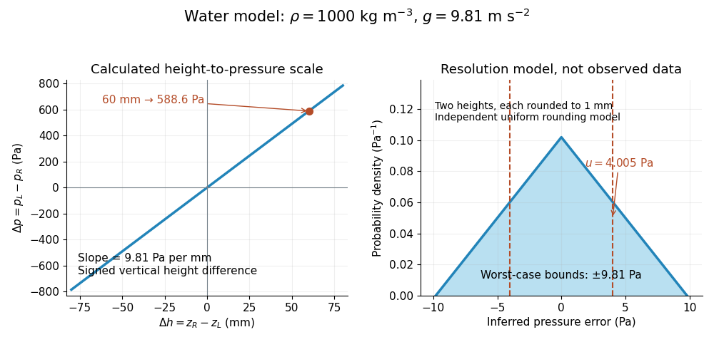
Suppose each liquid meniscus height is rounded to the nearest scale division $q=1\mathrm{mm}$. Each height measurement error lies within $q/2$, so the error in their difference lies within $q$. The resulting pressure error is bounded by $\rho gq=9.81\mathrm{Pa}$. To quantify a standard uncertainty, make the additional model assumption that the two rounding errors are independent random variables, each having a continuous uniform distribution on $[-q/2,q/2]$. Each then has variance $q^2/12$; adding the two variances givesHere $u$ denotes standard uncertainty. The $9.81\mathrm{Pa}$ worst-case bound and $4.0049\mathrm{Pa}$ standard uncertainty answer different questions. At $588.6\mathrm{Pa}$ they are respectively $1.67\%$ and $0.680\%$ of the reading. Shared reading bias or a different reading method can violate the assumed independence.

If the mass density, gravitational acceleration and height difference also have small independent standard uncertainties, a first-order estimate follows from the partial derivatives of $\Delta p=\rho g\Delta h$:This displays why a finer scale does not remove uncertainty in mass density or gravitational acceleration. A pressure transducer compared against the column needs its own differential-pressure calibration to establish an electrical response.

A mathematical model represents selected features of a system with mathematical objects and relations so that its behavior can be analyzed or predicted. Choosing the representation is part of the work: specify the quantities tracked, the equations or probability distributions connecting them, and the conditions under which those connections are expected to apply. A mathematical proof can establish a consequence of the model; comparing that consequence with observations tests its suitability for the intended use.

For a simple pendulum, the angle $\theta (t)$ and gravitational acceleration $g$ give the ideal equation $\ddot{\theta }+(g/\ell )\sin \theta =0$. Its assumptions include a point mass, fixed length $\ell$, uniform gravitational acceleration, and no damping. The small-angle approximation gives the simpler harmonic oscillator equation and oscillation period $T_0=2\pi \sqrt{\ell /g}$. A larger amplitude changes the full model's period; drag requires a damped pendulum. The simpler model remains useful when its omitted effects are small for the question being asked.

A model need not track every detail. A Bernoulli process models repeated success/failure observations using one probability and an independence assumption; a Gaussian process specifies a mean and a covariance function to model related measurements. Each representation enables calculations by retaining some distinctions and omitting others. Useful simplification therefore comes with a stated domain of use and quantities against which its predictions can be checked.

For an MPS tensor $A^i$, the transfer map is the completely positive map $\mathcal{E}(X)={\sum }_i{A}^{i}X(A^i{)}^{†}$. Its fixed points control normalization and local expectation values, while its subleading eigenvalues control correlation lengths.

For the normalized isotropic cutoff model, collisions redistribute the direction of relative velocity uniformly while keeping its length. With center $C=(v+v_{\ast })/2$ and relative speed $r=|v-v_{\ast }|$, outgoing velocities are $C\pm r\sigma /2$. Momentum and kinetic energy are preserved, and the collision rate has no relative-speed factor. The displayed operator uses unit total angular rate. General Maxwell molecule kernels can have nonconstant angular dependence.