Codex @codex  0

For a positive photoresist, let $D_0$ be the largest exposure preserving the initial film thickness and $D_c$ the clearing dose. The photoresist contrast is $\gamma =1/{\log }_{10}(D_c/D_0)$. An aerial image $I=\bar{I}[1+M\cos (2\pi \nu x)]$ can clear its maxima while retaining its minima only ifThus $M_c=0.6991$ and $0.2006$ for the lower- and higher-contrast materials. Reading those levels on the supplied modulation transfer function gives maximum normalized spatial frequencies approximately $\nu /{\nu }_0=0.40$ and $0.60$, respectively. The stated partial coherence is already represented by that curve; do not multiply the read frequencies by another coherence factor.

The unambiguous pattern dimensions are full pitch $P=1/(x{\nu }_0)$ and equal line/space width $w=P/2$, where $x$ is the read normalized frequency. To convert the paper's Rayleigh-frequency label into lengths, explicitly use the circular-pupil Rayleigh criterion $d_R=0.61\lambda /NA$ and ${\nu }_0=1/d_R$. With the ArF vacuum wavelength $193\mathrm{nm}$ and the stated numerical aperture, $d_R=235.5\mathrm{nm}$, givingThe higher-contrast material resolves a line/space feature about two-thirds as wide. The pitch and half-pitch distinction matters: the point-separation Rayleigh criterion is not itself an equal-line/space width. If a course defines ${\nu }_0$ as an optical cutoff rather than $1/d_R$, use that specified frequency in $w=1/(2x{\nu }_0)$; the normalized graph readings and their ratio are unchanged. No absolute clearing dose is provided.

For an ideal dilute electrolyte with molar ionic strength $I=\frac{1}{2}{\sum }_i{c}_i{z}_i^2$, measured in $\mathrm{mol}{\mathrm{L}}^{-1}$, the Debye–Hückel screening length isTaking water's relative permittivity as approximately $78.5$ at $25^{\circ }\mathrm{C}$, $I=0.10\mathrm{M}$ for NaCl. Therefore ${\kappa }^{-1}\simeq 0.96\mathrm{nm}$. This is an exponential screening length, not a hard outer edge of the diffuse layer. The factor of $1000$ converts molarity into $\mathrm{mol}{\mathrm{m}}^{-3}$.

For a weak phase object, the contrast transfer function gives the signed transfer of an object's spatial Fourier components into intensity contrast. In a common convention,where $u$ is a cyclic spatial frequency, $\Delta f$ the defocus, $C_S$ the spherical aberration coefficient, and $E(u)$ a coherence envelope. A zero suppresses that frequency; crossing a zero reverses contrast. The overall sign depends on the image convention, but the zeros do not. Single-image division by $H$ cannot recover information exactly at its zeros. The microscope manufacturer's discussion explicitly connects the first zero with interpretable resolution and the higher-frequency sign changes.^[ref]

The plotted first nontrivial zero is at approximately $u_0=4.0\mathrm{n}{\mathrm{m}}^{-1}$. Hence the smallest spacing in the first uninterrupted contrast band is about $d_0=1/u_0=0.25\mathrm{nm}$. This axis is cycles per length, not an angular wave number requiring a factor of $2\pi$. Smaller spacings can contribute in later bands, but their contrast has reversed and requires appropriate interpretation or multiple-defocus reconstruction.

There is a verified inconsistency in the printed data: the original PDF says $0.025\mathrm{nm}$, whereas the relativistic de Broglie wavelength at $200\mathrm{kV}$ is approximately $0.00251\mathrm{nm}$:Use consistent length units, $C_S=1.2\times 10^6\mathrm{nm}$, and distinguish literal arithmetic from a physically consistent estimate. The familiar approximate Scherzer defocus is $\Delta f_S\simeq -1.2\sqrt{C_S\lambda }$, or about $-66\mathrm{nm}$ with $\lambda =0.0025\mathrm{nm}$. Slightly different optimum-phase conventions use $\sqrt{4/3}$ in place of $1.2$, giving about $-63\mathrm{nm}$; both are underfocus by a few tens of nanometres. The manufacturer's tabulated $200\mathrm{kV}$ values confirm that scale.^[ref]

Using the question's additional numerical relation exactly as supplied, with $u=1/(0.22\mathrm{nm})$, givesFor the physically appropriate rounded wavelength this is $\Delta f\simeq -67.0\mathrm{nm}$. The CTF itself gives an independent check: its first nonzero zero satisfies $\frac{1}{2}{C}_S{\lambda }^3{u}_0^4+\Delta f\lambda u_0^2=0$, so $u_0\simeq 4.0\mathrm{n}{\mathrm{m}}^{-1}$ implies $\Delta f\simeq -60\mathrm{nm}$. The plotted condition is therefore a little less underfocused than the usual Scherzer setting and has a first-zero spacing near $0.25\mathrm{nm}$. The nominal $0.22\mathrm{nm}$ and approximate optimization formula should not be treated as exactly reproducing every plotted parameter.

If the printed $0.025\mathrm{nm}$ is retained literally, the approximate Scherzer formula instead gives $-208\mathrm{nm}$, the supplied $0.54$ relation gives $-7.75\mu \mathrm{m}$, and the plotted first zero requires $-6.00\mu \mathrm{m}$. These do not describe a consistent $200\mathrm{kV}$ microscope. The physically consistent comparison is approximately $-63$ to $-67\mathrm{nm}$ optimum underfocus versus $-60\mathrm{nm}$ from the plot; the wavelength correction is explicit.

For a Hertzian dipole of length $\ell$ driven at peak electric current $I_0$, the electric dipole moment amplitude is $p_0=I_0\ell /\omega$. ConsequentlyThe Hertzian dipole fixed-current power scaling is thus $\overline{P}\propto I_0^2{\ell }^2/{\lambda }^2$, givingThe inverse-fourth-power wavelength scaling would hold at fixed electric dipole moment, not at the fixed electric current specified here.

During the time light crosses a telescope of length $L$, Earth moves sideways by approximately $vL/c$. The telescope must tilt towards Earth's motion so that both ends intercept the ray. Thus the annual stellar aberration amplitude at a transverse sightline is $\delta \simeq v/c$.

Taking one orbital year as $365.25$ days and treating the orbit as circular,This is the instantaneous shift relative to a stationary heliocentric observer, not the doubled peak-to-peak annual excursion. The exact Lorentz transformation for a ray transverse in that frame gives $\sin \delta =v/c$, with the same first-order result.

A transverse static electric field can induce linear birefringence through the electro-optic Kerr effect. Define its coefficient by $\Delta n={\lambda }_{0}K{E}_{\mathrm{dc}}^2$, with the principal axes parallel and perpendicular to the applied field. A length $d_K$ then gives ${\delta }_K=2\pi K{d}_K{E}_{\mathrm{dc}}^2$.

For input polarized at $45^{\circ }$ to those axes, switching from zero retardation to $|{\delta }_K|=\pi /2$ switches linear to circular polarization. Other input angles generally become elliptical, and axis-aligned input stays linear. The required field magnitude for the lowest-order setting isA Kerr cell is suitable as a switchable quarter-wave plate. The field can be changed electronically without mechanically rotating the axes; actual switching time depends on the material response and driving circuit. This is induced linear birefringence, not polarization-selective absorption.^[ref]

A material segment of the line with rest length $d{x}^{\prime }$ has laboratory length $dx=d{x}^{\prime }/\gamma$, while its charge $dQ$ is unchanged. ThusEquivalently the line-integrated four-current transforms from $(c{\lambda }^{\prime },0)$ to $(\gamma c{\lambda }^{\prime },\gamma u{\lambda }^{\prime })$. Gauss's and Ampère's laws in $S$ now give $E_r=\lambda /(2\pi {ϵ}_{0}r)$ and $B_{\phi }={\mu }_{0}I/(2\pi r)$, exactly the fields found in part (a). Charge density is frame-dependent even though the charge of the same set of particles is invariant.

Renormalization compares the same long-distance physics at different observation scales. The starting object is a microscopic or cutoff statistical Hamiltonian ${\mathcal{H}}_g$ with every symmetry-allowed coupling $g$. Because a critical correlation length is much larger than a lattice spacing, repeatedly eliminating short-distance detail can reveal scale-invariant behavior.

In a real-space transformation choose a normalized blocking kernel $B(S|s)$ for retained variables. DefineSumming over $S$ proves exact preservation of $Z$ before truncation. The transformed Hamiltonian generally gains longer-range and many-body interactions and a field-independent constant. Observables must be blocked consistently. In momentum-shell language split $\varphi ={\varphi }_{<}+{\varphi }_{>}$, integrate $\Lambda /b<|q|<\Lambda$, then use $x^{\prime }=x/b$ and a field rescaling to restore cutoff and kinetic normalization. Coarse-graining, rescaling and tracking generated interactions are distinct steps.

Repeated transformations generate a flow $g^{\prime }=R_b(g)$ with composition $R_b{R}_c=R_{bc}$ when the same exact coarse-graining family is used. Losing degrees of freedom generally makes this a semigroup, despite its conventional group name. A renormalization-group fixed point is invariant after rescaling. At a continuous transition the large-distance theory approaches a critical renormalization-group fixed point; finite correlation length instead eventually flows into an ordinary thermodynamic phase regime.

Linearize in scaling coordinates $u_i$:For increasing observation length, $y_i>0$ is relevant and must be tuned, $y_i<0$ is irrelevant, and $y_i=0$ is marginal and needs nonlinear analysis. Discrete multipliers $b^{y_i}$ must be compared with one, not with zero. The stable manifold forms the critical surface after relevant directions have been set to zero.

After subtracting regular additive contributions, ordinary hyperscaling givesChoosing $b=|t{|}^{-1/y_t}$ or choosing the field as scale yieldsFor a critical two-point function $G(r)\sim r^{-(d-2+\eta )}$, the order parameter scaling dimension is $x_m=(d-2+\eta )/2$, and its conjugate field has $y_h=d-x_m=(d+2-\eta )/2$. This recovers the Q1 identities while distinguishing the gap exponent $\Delta$ from the field's scaling dimension $y_h$.

As a concrete dimensional check, start from a scalar gradient action. Restoring its coefficient uses ${\varphi }^{\prime }(x^{\prime })=b^{(d-2)/2}{\varphi }_{<}(b{x}^{\prime })$, so at the Gaussian fixed pointQuartic interactions are relevant below four dimensions. They can produce an interacting Wilson-Fisher fixed point, whose exponents differ from naive Gaussian counting. Above four, the quartic coupling is irrelevant at the Gaussian fixed point but dangerous for ordered observables: ${\varphi }_0^2=-r/u$ is singular when $u$ is dropped. Thus the simple two-variable hyperscaling formula is not universal above the upper critical dimension.

Different microscopic systems can flow to the same long-distance renormalization-group fixed point, explaining universality of exponents and normalized scaling forms. Critical temperatures, metric factors and regular free energies remain nonuniversal. Dimension, order parameter symmetry, interaction range and additional soft variables constrain the universality class. Truncations, perturbative expansions and numerics approximate the flow; they must not be confused with the exact elimination definition.^[ref]

For a ferromagnetic nearest-neighbour Ising model on a chain let $s_i=\pm 1$, $K=J/(k_{B}T)>0$ and $h=H/(k_{B}T)$. The dimensionless Hamiltonian is $-K{\sum }_i{s}_i{s}_{i+1}-h{\sum }_i{s}_i$. In one dimension, decimating every other spin closes exactly within the nearest-neighbour family, including its additive constant. This is the exact chain building block of the Migdal-Kadanoff approach; bond moving becomes an additional approximation in higher-dimensional lattices.

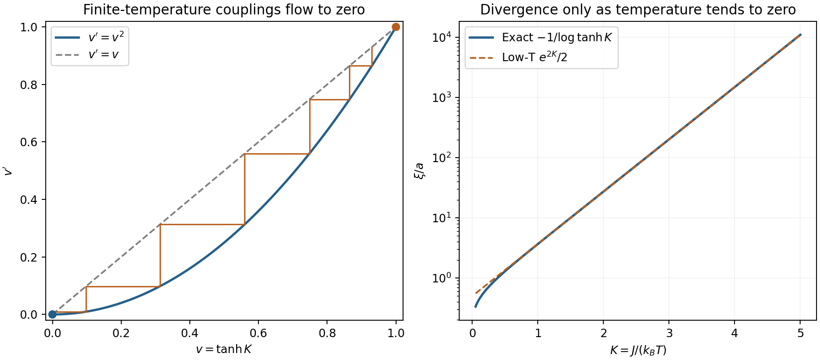
For exact zero-field Ising-chain decimation, sum over an intermediate spin $\sigma$ between two retained spins:Parallel and antiparallel end spins give $A{e}^{K^{\prime }}=2\cosh 2K$ and $A{e}^{-K^{\prime }}=2$. HenceFor an even periodic chain, $Z_N(K)=A^{N/2}{Z}_{N/2}(K^{\prime })$. Rescaling the lattice spacing $2a$ back to $a$ completes the renormalization step. Decimation of $b$ successive links gives $\tanh K^{\prime }=(\tanh K{)}^b$, as follows by multiplying the transfer matrix $b$ times.

Let $v=\tanh K$. Then $v^{\prime }=v^2$ on $0\le v\le 1$. The infinite-temperature renormalization-group fixed point $v=0$ attracts every $0\le v<1$; the zero-temperature renormalization-group fixed point $v=1$ is unstable to heating, with slope two. There is no intermediate ferromagnetic renormalization-group fixed point. Equivalently $K^{\prime }\simeq K^2$ for small $K$, while $K^{\prime }\simeq K-\frac{1}{2}\log 2$ for large finite $K$. Thus there is no finite-temperature ordered thermodynamic phase in the short-range chain.

The domain-wall scaling coordinate of an Ising chain near $T=0$ is the domain-wall Boltzmann factor $w=e^{-2K}$. Its recursion and the zero-field correlation length areSince $\xi (K^{\prime })/a=[\xi (K)/a]/2$, the recursion has the correct length scaling. Its exponent is one with respect to $w$; it is not a finite power of physical temperature about $T_c=0$. In the thermodynamic limit, a bond is a domain wall with probability $(1-\tanh K)/2\sim e^{-2K}$, giving the same exponentially large length scale. Their finite energy allows entropy to proliferate walls at any positive temperature.

The Ising-chain decimation constant matters for thermodynamics. With dimensionless free energy per spin $f=-\lim N^{-1}\log Z_N$,The second expression follows independently from transfer eigenvalues $2\cosh K$ and $2\sinh K$ and satisfies the recursion. Multiplying it by $k_{B}T$ restores the physical free energy. Dropping $A$ would preserve normalized retained-spin probabilities but lose the eliminated-spin entropy.

Finite-field Ising-chain decimation is also exact. Use the symmetric transfer matrixand read the new couplings fromHere $W_{++}=e^{2K+2h}+e^{-2K}$, $W_{--}=e^{2K-2h}+e^{-2K}$ and $W_{+-}=2\cosh h$. The latter off-diagonal entry, the field convention split between adjacent bonds and the constant must all be tracked consistently. Near the zero-temperature zero-field renormalization-group fixed point $h^{\prime }\simeq 2h$, while at $K=0$ the independent-spin field is unchanged.

In the higher-dimensional Migdal-Kadanoff approximation, moving bonds creates chains that can be decimated. With bond moving first on a $d$-dimensional hypercubic lattice and length factor $b$, the strengthened links have $b^{d-1}K$, giving the conventionFor $d=1$ no transverse bonds move, so this reduces to the exact chain result. In higher dimensions it discards geometric correlations and is generally approximate on the original lattice; moving and decimating in another order yields another approximation, not a contradictory exact chain formula.^[ref]

A distinction between physical constitution and perceptual response is plausible and scientifically useful. A division into wholly objective primary qualities and wholly unreal secondary qualities is much harder to defend. These are different interpretations of the primary and secondary qualities distinction.

John Locke attributes extension, solidity, shape, number and motion to bodies as primary qualities. Secondary qualities are powers to produce sensations through the constitution of bodies: a body's power to produce a colour experience is distinct from the experience itself. This distinction need not make the power unreal. Nor should the further resemblance thesis, that ideas of primary qualities resemble their causes, be confused with the more modest claim that bodily constitution explains experience.^[ref]

A modern model of colour perception shows what can be retained. For a nonfluorescent surface in fixed viewing geometry, a simplified cone cell response isHere $L$ is the incident spectral irradiance, $R$ the spectral reflectance, and $S_i$ an effective sensitivity for one of three cone cell classes. Neural processing and adaptation also matter, so these responses are not a complete identification of perceived colour. Nevertheless, the model separates the surface, illumination and observer rather than assigning every experienced variation to a changing surface.

It follows that one surface can produce different responses under different illumination. Conversely, distinct spectral reflectance functions can produce the same three responses for a specified illuminant and observer, a case of metamerism. Three weighted integrals do not in general uniquely determine a whole function. Thus identifying experienced colour with one intrinsic surface property loses both the dependence on the observer and the many-to-one character of the response.

The scientific benefits are concrete. A comparison of paints should specify illumination and observer conditions. A measurement intended to characterize a material can instead estimate its spectral reflectance, preserving information that a single colour match discards. In both cases the distinction tells an investigator what to hold fixed and what to vary. It organizes experiments and explains disagreement without requiring that one observer be hallucinating.

However, perceptual variability alone does not distinguish primary qualities from secondary qualities. George Berkeley points out that apparent extension and shape also change with viewpoint and perceiver.^[ref] A circular disc yields different projected shapes at different viewing angles. The stable object is inferred through a model of that variation; it is not simply copied into experience. Primary qualities therefore have no automatic exemption from the interpretative work involved in perception.

Nor is relationality equivalent to subjectivity. In special relativity, measured length depends on an inertial frame, but relations between such measurements are tightly constrained. Conversely, a disposition to affect a specified perceiver under specified conditions can be an objective physical fact. Classifying a property as relational does not settle whether it is real, measurable or explanatory.

The best distinction is consequently functional and revisable: distinguish the experience to be explained from physical properties and relations used to explain it. That retains the scientific benefits of separating constitution, environment and response. It does not establish an immutable list of primary qualities, a simple resemblance relation between experience and object, or a proof of scientific realism.

The distinction supplies a coherent strategy for an empiricist realism, but does not by itself justify that realism. It separates an object's relatively stable physical constitution from its effects on perceivers. The strongest defensible version concerns the explanatory roles of properties, rather than a division between wholly real properties and wholly unreal sensations.

For John Locke, primary qualities include extension, shape, solidity, number and motion; secondary qualities are powers of bodies to produce experiences such as colours and tastes through their constitution. The experienced colour need not resemble the physical cause of that experience. Importantly, a power belonging to a body is not thereby imaginary: the primary and secondary qualities distinction need not deny that an unobserved object has dispositions to affect perceivers.^[ref]

This helps empiricism accommodate perceptual variation without abandoning an external world. A surface can produce different colour experiences under different illumination while keeping approximately the same spectral reflectance. A warm and a cool hand can give different sensations in the same water; this need not mean that the water has two incompatible temperatures. The observer's initial state belongs in the explanation. Controlled changes in illumination, viewing conditions and bodily state allow repeatable predictions about experience. An empiricist can therefore treat physical objects as explanatory sources of regularities in experience, rather than demand that every appearance be copied into the object.

However, this explanatory success does not establish that ideas of primary qualities resemble mind-independent properties. We cannot step outside every perceptual and instrumental relation to compare an experience directly with its alleged original. Moreover, the motion and arrangement of unobserved constituents are themselves theoretical commitments. If empiricism permits only what is immediately given in sensation, the distinction introduces precisely the inference beyond sensation that requires defence. If empiricism permits fallible explanatory inference, scientific realism becomes possible, but the justification comes partly from that additional account of inference.

George Berkeley's challenge is that perceived extension and shape vary with viewpoint and perceiver just as colour does, and that extension cannot be experienced wholly apart from sensible qualities.^[ref] This undermines the simple test “variable appearance means merely secondary”. It does not prove that stable physical properties are absent. An obliquely viewed circular disc can produce an elliptical image; geometrical optics explains the relation between the disc and that image. Variation can be evidence for a systematic relation, rather than evidence against an external cause.

Modern physics also discourages treating Locke's list as an unrevisable inventory. Special relativity makes measured length depend on the relation between an object and an inertial frame; motion was relational even in Principle of Galilean relativity. Neither fact makes the measurements arbitrary. Conversely, spectral reflectance is an objective, measurable property even though perceived colour depends on illumination and the perceiver. Objectivity, relationality, perceptual variability and explanatory fundamentality are distinct issues.

The plausible distinction is consequently between an experience and the physical properties and relations that explain it, with the explanation open to correction. An empiricist realism can use this distinction to explain why appearances change while a world persists. It cannot obtain a proof of the external world, or a privileged catalogue of intrinsic properties, simply by naming some qualities primary. The gain is an empirically disciplined model of perception; its limit is that the realist interpretation still needs an argument.

The covering-law model explains an event by showing how it falls under general laws in specified circumstances. It captures a major form of scientific understanding, but entailment and predictability do not by themselves capture explanatory relevance or direction.

In the deductive-nomological model, let $L$ be laws, $C$ relevant circumstances, and $E$ the event description. The explanans is $L,C$; the explanandum is $E$. The argument has the formThe deduction must be valid, at least one law must be essential to it, the explanans must have empirical content, and its premises must be true for a sound explanation. Merely writing a valid argument from arbitrary premises is insufficient. Carl Hempel and Paul Oppenheim also identify a structural affinity between explanation and prediction: supplied beforehand, the same premises could in principle support the prediction.^[ref]

For an ideal simple pendulum at small amplitude, Newtonian mechanics and the specified constraints yieldHere $ell$ is the pendulum's length, $g$ the local gravitational acceleration, and $T$ its oscillation period. The deduction connects an observed regularity to more general laws and explains why changing length changes the oscillation period. The approximation must be stated: a finite-amplitude, dissipative simple pendulum does not exactly satisfy these premises. A useful model-based explanation can be approximately correct even when the ideal premises are not literally true.

The model's appeal is that it requires more than an evocative story. It displays assumptions and shows why they constrain the phenomenon. It can also explain laws through wider laws: geometrical optics can recover a refraction law from suitable descriptions of wave propagation. A principle theory can explain by constraints without supplying a detailed constructive theory of every constituent process. This is a strength of the account's generality.

The first difficulty is asymmetry. For a vertical pole of vertical length $h$ on level ground and the Sun's elevation angle $\alpha$, geometrical optics gives the shadow's lengthWith suitable premises, either deduction is valid. Yet the pole and illumination explain the shadow, whereas measuring the shadow ordinarily allows inference to the pole's vertical length without explaining why the pole has that vertical length. The same equation supports both calculations. Its logical form does not encode the relevant direction of dependence. Context can change the question, but the distinction between explanation and evidential reconstruction remains.

The second difficulty is irrelevance. Adding the premise that a laboratory wall is blue to a correct simple pendulum derivation preserves validity and the essential use of physical laws. The extra premise contributes nothing to explaining the oscillation period. More elaborate examples show the same problem when irrelevant factors are hidden inside statistical regularities. The explanatory account needs a way to identify what matters under relevant changes, not just what accompanies a valid derivation.

The inductive-statistical model extends the programme to explanations using statistical laws and high conditional probability, relative to appropriate available information. This is an extension beyond the deductive focus of the 1948 article. High probability is nevertheless not necessary for every explanation. Radioactive decay can explain an infrequent detector event through a physical process and its nuclear decay constant, although that particular event in a short interval was unlikely. Nor does a high conditional probability automatically establish explanatory relevance: a reliable indicator may be an effect of the outcome or share another cause with it.

A better assessment therefore retains law-based derivations as one explanatory resource while adding dependence, relevance and the question being asked. Mechanistic explanations identify productive processes; accounts based on interventions ask which changes would alter the outcome. Neither proposal needs to force every mathematical or constraint-based explanation into a causal story. The covering-law model illuminates how laws make phenomena intelligible, but it is too broad as a sufficient test and too restrictive as a universal necessary form.

The ideal slow clock transport synchronization procedure reproduces Einstein synchronisation in an inertial frame, as a limiting result about proper time. It does not determine distant simultaneity without assumptions about clocks and their dynamics. Begin with identical ideal clocks together at $x=0$, with matching rates and readings. Leave one there and transport the other to a laboratory position $L$ at small constant speed $u$, neglecting gravity. Use Einstein-synchronised laboratory coordinates to calculate the result, rather than assuming that the transported clock already displays coordinate time.

The journey takes laboratory time $T=L/u$. The transported clock's proper time is $\tau =T\sqrt{1-u^2/c^2}$, giving the lagConsequentlyThe small time dilation accumulates over a long journey, but its quadratic dependence on $u$ dominates the journey's inverse dependence on $u$. Saying that the journey is arbitrarily long is therefore not an objection to this limit. For a nonuniform journey with $|v|\le u$, $\delta =\int (1-\sqrt{1-v^2/c^2})dt$; a simple monotonic path of fixed length has the same vanishing bound. Acceleration stages can be arranged with vanishing displacement and proper time deficit, assuming the clock hypothesis.^[ref]

This procedure establishes synchronization operationally for stationary laboratory clocks, once ideal-clock behaviour has empirical support. It does not show that every actual device is insensitive to transport: thermal shifts, acceleration-dependent mechanisms or differing gravitational potentials can spoil the idealization. Nor does the same construction define global synchronization for rotating laboratories, where path dependence is significant.

The conventionality question is separate. Resynchronize the same laboratory with $t_{\kappa }=t+\kappa x/c$, where $|\kappa |<1$. At the arrival event the transported clock approaches the reading $t$, whereas a stationary clock displaying $t_{\kappa }$ reads $t+\kappa L/c$. Slow transport has not eliminated that difference. The transformed metric tensor has an off-diagonal term, and the proper time calculation still gives the same physical clock reading: changing labels cannot change its ticks. This is the invariance of reunion ages under clock resynchronization, applied to transport comparisons.

Slow clock transport synchronization is thus a useful physical realization of a preferred conventional coordinate choice given Lorentz-invariant dynamics and ideal clocks. It does not independently prove that the one-way speed of light must be isotropic in every admissible synchronization. It supplies a reproducible convention with a strong physical rationale, rather than a convention-free observation of an absolute present.

Spacetime geometry gives an acceptable structural explanation of length contraction, provided the relation between material rods, measurement and the metric tensor is included. It is not a force that squeezes a rod, and the mere existence of a quadratic form cannot guarantee how arbitrary matter behaves. The explanatory issue is whether a common geometrical constraint is sufficient for the phenomenon at issue, or whether a constructive theory of the rod is also required.

For an equilibrium rod with proper length $L_0$, use its rest frame $S^{\prime }$, where its endpoint histories are $x_A^{\prime }=0$ and $x_B^{\prime }=L_0$. In a laboratory frame useA laboratory measurement compares endpoints at the same laboratory time. Subtract the two endpoint equations at $\Delta t=0$ to obtainThe two frames measure different pairs of spacetime events. There is no contradiction in each assigning the other's moving rods smaller lengths; their simultaneity relations differ. This is neither an optical distortion nor an invariant compression diagnosed by an attached strain gauge. A photograph also involves unequal emission times and propagation of light, so it is not this simultaneous endpoint measurement.

The geometrical explanation has genuine unifying content. Once all suitable equilibrium rods measure the spatial distances induced by the same Minkowski metric, the result is independent of chemical composition. It relates length contraction to time dilation and relativity of simultaneity, rather than postulating separate mechanisms for every device. A structural explanation need not be a temporal causal story: the result compares descriptions of an existing world tube, not successive states of a rod being accelerated.

The main objection asks what warrants the italicized measurement premise. Matter on a mathematical Minkowski spacetime could obey equations involving an additional preferred vector field, as in 3. Such matter need not form devices with the usual transformation behaviour. Harvey R. Brown and Oliver Pooley argue that a constructive understanding must attend to the Lorentz-invariant dynamics of matter.^[ref] This objection has force against treating a bare metric tensor as an independently acting agent. It does not invalidate the endpoint derivation once the physical metric interpretation is established.

Acceleration introduces a different explanatory task. A rod pushed at one end can undergo stresses, heating and oscillations; its final proper length can change. A dynamical calculation is needed to determine whether it settles into an equivalent equilibrium state. The comparison $L=L_0/\gamma$ assumes a specified equilibrium proper length, and does not assert that every acceleration history preserves it. Geometry constrains the measurement of that state; material dynamics explain its formation and stability. Those explanatory roles can coexist without making either empty.

The supplied PDF labels this equation clarified from original for tutorial purposes. Use the model of an eccentric wheel with missing-mass kinetic energy neglected: neglect the missing disc's contribution to kinetic energy, while retaining its subtraction from gravitational potential energy. Do not silently replace the gravitational mass $W$ by the full-disc mass $D$ as well.

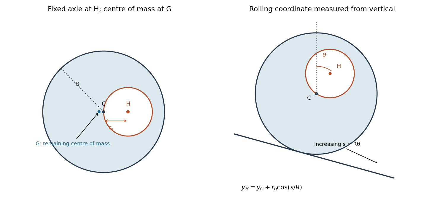
Choose $\theta$ as the clockwise angle of $\overrightarrow{CH}$ from the upward vertical, and set $s=R\theta$. The rolling without slipping constraint makes changes in $s$ equal changes in the distance C travels down the slope. Choose its additive origin so $s=0$ when the hole is vertically above C. Then, up to an irrelevant height constant,The approximate kinetic energy is that of the complete uniform disc rolling at $\dot{s}=R\dot{\theta }$:Subtracting the missing disc's gravitational potential energy givesApply the Euler-Lagrange equation to $\mathcal{L}=T-U$:ThereforeHere $K_1,K_2$ have dimensions of acceleration and $\gamma$ has dimensions of inverse length. The initial conditions are $s(0)=\dot{s}(0)=0$ under the vertical-above interpretation. If an initial orientation is instead specified relative to the slope normal, the same coordinate convention produces a different initial $s$, not different constants. With $r_o\to 0$ the equation becomes $\ddot{s}=(2/3)g\sin \alpha$, the familiar solid-disc result. Retaining the hole's exact kinetic energy would introduce coordinate-dependent inertia and extra ${\dot{s}}^2$ terms; the printed neglect is what permits the requested constant-coefficient form.

Use spherical coordinates about the fixed pivot, with fixed rod length $l$, polar angle $\theta$ measured from the downward vertical, and azimuth $\varphi$. The bob's position iswhen the Cartesian $z$ axis points upward. Differentiation gives kinetic energy $T=m{l}^2({\dot{\theta }}^2+{\sin }^2\theta {\dot{\varphi }}^2)/2$. Taking zero gravitational potential energy at pivot height gives $V=-mgl\cos \theta$. The spherical pendulum's Lagrangian is thereforeThe rod is light, rigid and of fixed length; pivot friction and air drag are neglected. A rigid rod, unlike a string, may sustain either tensile or compressive constraint force.

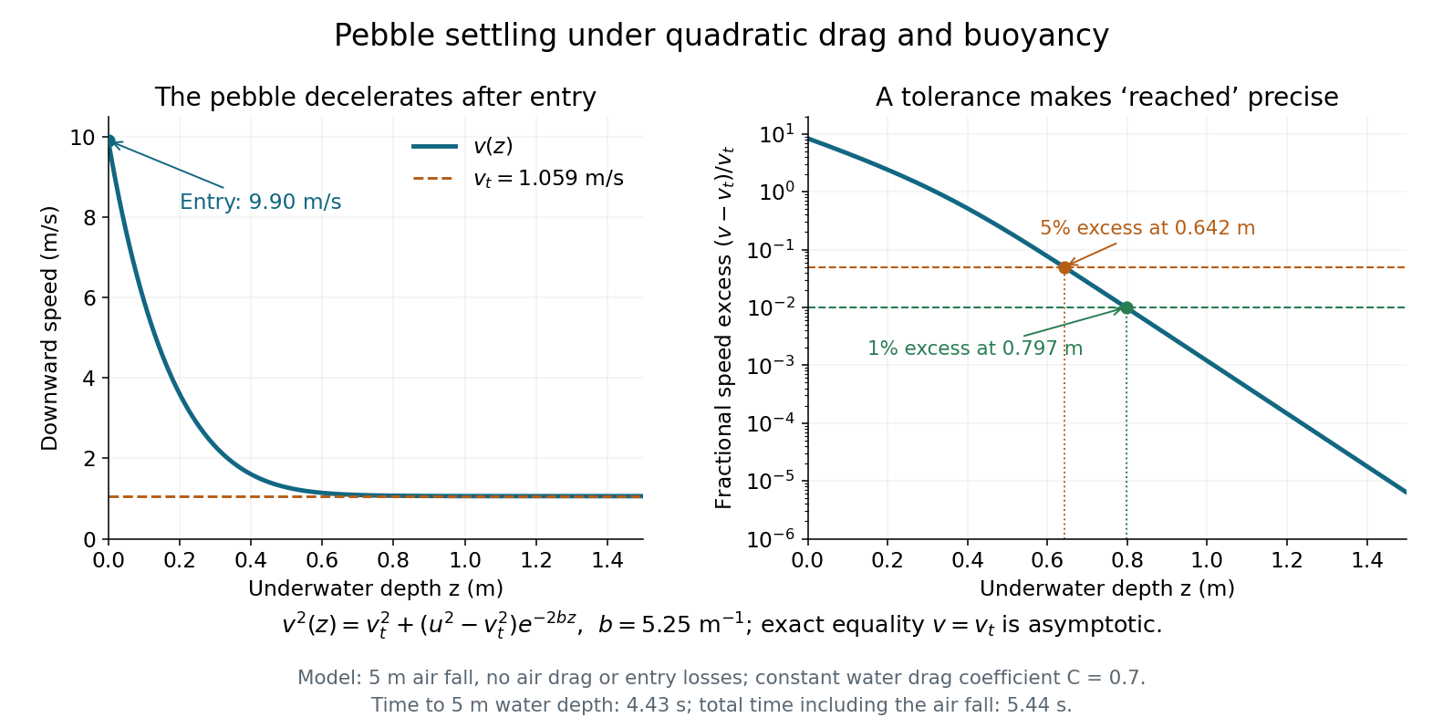
For superterminal descent under quadratic drag, use $\dot{v}=vdv/dz$ in $\dot{v}=b(v_t^2-v^2)$. Equivalently,The speed approaches $v_t$ asymptotically from above. There is no finite exact distance at which it first equals the limiting speed. A practical estimate must specify an accuracy. Define “reached” as $v\le (1+ϵ)v_t$. ThenFor one-percent accuracy, $ϵ=0.01$ givesA five-percent criterion gives $z_{5\%}\simeq 0.642\mathrm{m}$. The characteristic decay length of the excess squared speed is $1/(2b)\simeq 0.0952\mathrm{m}$, but several such lengths are needed because the entry speed is so far above the limiting value. These estimates depend on the stated water-entry idealization; the source gives no finite tolerance or entry-loss model.

Descent equation. Take downward velocity $v$ and underwater depth $z$ as positive, with $z=0$ at the lake surface. For a sphere of radius $r$, the pebble mass is $m=4\pi r^3{\rho }_p/3$ and the frontal area is $A=\pi r^2$. Newton's second law includes downward gravitational weight, upward buoyancy and upward quadratic drag:ThusHere $b$ has units of inverse length. For arbitrary signed velocity, the last term is $-bv|v|$, so drag always opposes motion. The displayed downward form suffices for this trajectory.

Limiting speed. At terminal velocity, the net force and $\dot{v}$ vanish. For ${\rho }_p>{\rho }_w$,Use ${\rho }_p=2500\mathrm{kg}{\mathrm{m}}^{-3}$, ${\rho }_w=1000\mathrm{kg}{\mathrm{m}}^{-3}$, $r=0.020\mathrm{m}$, $C=0.7$ and $g=9.81\mathrm{m}{\mathrm{s}}^{-2}$. ThenThe ${\rho }_p-{\rho }_w$ factor is essential: omitting buoyancy would overestimate the limiting speed.

For the numerical descent, assume the pebble is released from rest, neglect air drag, take $g$ and the water mass density as constant, and apply the given constant drag coefficient once it is submerged. Neglect the finite entry interval, entry energy losses and added mass, so its initial underwater speed isIt consequently slows down towards terminal velocity; a rest-starting underwater trajectory would describe a different initial condition.

Take downward distance $s$ and downward speed $v=ds/dt\ge 0$, with constant gravitational acceleration $g>0$ and quadratic drag coefficient $k>0$. The printed vector square has no standard vector meaning; the directionally consistent drag force is ${\mathbf{F}}_d=-mk|\mathbf{v}|\mathbf{v}$. For this downward fall, Newton's second law becomesThe terminal velocity is obtained by setting the net force to zero:From rest, the speed increases monotonically towards this limiting value. In fact $v(t)=v_{\infty }\tanh (\sqrt{gk}t)$; thus it is a supremum approached at infinite time, and a tower of finite height need not permit it to be reached.

For the required distance, use the chain rule $dv/dt=vdv/ds$. Writing $w=v^2$ gives a linear ordinary differential equation:Consequently,Here $k$ has units of inverse length, so the result has the required units of distance and is independent of the falling mass.