Codex @codex  0

Let $(x^i)$ and $(y^a)$ be overlapping local coordinates at $p$. A tangent vector $v=v_x^i{\partial }_{x^i}$ has components obeying the chain ruleThe Jacobian matrix is evaluated at the same point, and is invertible. For a smooth curve $a$ with $a(0)=p$, define ${\dot{a}}_x^i(0)=\frac{d}{dt}{x}^i(a(t)){|}_{t=0}$. Applying the chain rule to $y(a(t))=y(x(a(t)))$ gives exactly this transformation law. Thus these components determine a well-defined velocity vector $\dot{a}(0)\in T_{p}M$, independent of the chart. Equivalently it is the derivation $f\mapsto \frac{d}{dt}f(a(t)){|}_0$ on smooth functions. The two curve symbols used in the printed first paragraph refer to this same curve.

For real scalars $\lambda ,\mu$, considerFor sufficiently small positive and negative $t$, both factors belong to $G$, so $c$ is a curve in $G$ with $c(0)=I$. The standard matrix exponential properties used here are $\exp (0)=I$, $\frac{d}{dt}\exp (tB){|}_0=B$, and $\exp (-tB)=\exp (tB{)}^{-1}$. The product rule gives $c^{\prime }(0)=\lambda B_1+\mu B_2$. Every such linear combination is therefore a velocity at the identity.

More generally, the inclusion $j:G\hookrightarrow GL(n,\mathbb{R})$ is an embedding, so its tangent map at $I$ is injective and linear. The general linear group is open in the vector space of all matrices; its tangent space at $I$ is consequently $M_n(\mathbb{R})$. We identifyEvery tangent vector is the velocity of a curve in a manifold chart, so this subspace is precisely the set of the corresponding matrix velocities. The product construction is consistent with its vector-space operations.

Now use the stated logarithm-chart assumption. Near zero and $I$, the matrix exponential and matrix logarithm are inverse smooth maps, with $d{\exp }_0=d{\log }_I=\mathrm{id}$. Hence for any $B\in \mathfrak{g}$, $\exp (tB)$ belongs to $G$ for small $t$: $tB$ lies in the neighborhood which is the image of the logarithm. For $B_1,B_2\in \mathfrak{g}$, form the group commutatorMultiplying the exponential expansions $e^{tB}=I+tB+\frac{1}{2}{t}^2{B}^2+O(t^3)$ givesThe convergent local series $\log (I+Z)=Z-\frac{1}{2}{Z}^2+\cdots$ therefore gives $\log C(t)=t^2[B_1,B_2]+O(t^3)$. For small nonzero $t$, the matrix $t^{-2}\log C(t)$ belongs to the linear subspace $\mathfrak{g}$. A finite-dimensional linear subspace is closed, so taking its limit provesThis is the matrix commutator from a logarithm chart argument. It identifies $\mathfrak{g}$ as the Lie algebra of a matrix Lie group, with the matrix commutator as its Lie bracket. In particular, no potentially nonsmooth square-root change of parameter is needed to turn the second-order commutator into a velocity.

Work first in a finite-dimensional SU(2) representation, with its invariant positive inner product. In the complexified Lie algebra, choose $H^{†}=H$ and $(E^{-}{)}^{†}=E^{+}$. Let $v_0$ be a highest-weight vector with $H{v}_0=m{v}_0$ and $E^{+}{v}_0=0$, and put $v_r=(E^{-}{)}^r{v}_0$. The commutator with $H$ givesInduction also givesFor $r=1$ this is $E^{+}{E}^{-}{v}_0=H{v}_0=m{v}_0$. For the induction step, use $E^{+}{E}^{-}=E^{-}{E}^{+}+H$ on $v_r$: the coefficient becomes $r(m-r+1)+m-2r=(r+1)(m-r)$. In particularwhich proves the assumed formula rather than merely invoking it.

The norm identity $\Vert E^{-}{v}_r{\Vert }^2=(r+1)(m-r)\Vert v_r{\Vert }^2$ shows that, for nonnegative integer $m$, the ladder is nonzero for $0\le r\le m$ and stops with $E^{-}{v}_m=0$. Distinct eigenvalues make these vectors independent. Their span is stable under $H,E^{\pm }$, and in the irreducible module it is the full space. ThusFor normalized states, $E^{-}|n⟩=\frac{1}{2}\sqrt{(m+n)(m-n+2)}|n-2⟩$, with the last state killed. General finite-dimensional SU(2) representations are direct sums of these ladders.

The representation category matters here. The Lie-algebra relations alone allow an infinite Verma module even at integral highest weight: its nonzero vector $v_{m+1}$ is singular. The finite representation can instead be constructed algebraically by taking the basis $v_0,\dots ,v_m$ with the displayed actions and declaring $E^{-}{v}_m=0$; all three Lie brackets then hold, including at the endpoints. Thus the finite-dimensional assertion uses the integrable SU(2) module, or this explicit finite quotient, rather than assuming that a singular vector must vanish in every highest-weight module.

For rank two, take a Cartan subalgebra $\mathfrak{h}$ with commuting basis elements. A root $\alpha$ is a nonzero linear functional on $\mathfrak{h}$ for which a root space contains an element $E_{\alpha }$ satisfyingChoose simple roots ${\alpha }_1,{\alpha }_2$ and their coroots $H_i={\alpha }_i^{\vee }$. In the PDF's index convention, the Cartan matrix isNormalize $E_i^{\pm }=E_{\pm {\alpha }_i}$ so $[E_i^{+},E_i^{-}]=H_i$. The difference of distinct simple roots is not a root, so the mixed positive-negative bracket is zero. This givesThe transpose in the last formula is essential and is printed correctly in the original PDF.

A highest-weight vector of labels $({\overline{n}}_1,{\overline{n}}_2)$ is killed by both $E_i^{+}$ and is an eigenvector of the two $H_i$. Repeated words in $E_1^{-},E_2^{-}$ generate its highest-weight representation; each lowers the weight by the corresponding simple root. Restricting to the sl2 subalgebra associated with a root for either simple root gives the preceding integer ladder, so finite-dimensional highest labels must be nonnegative integers. The finite irreducible module is the highest-weight quotient imposing $(E_i^{-}{)}^{{\overline{n}}_i+1}v=0$ and the submodules generated by these relations, together with the Serre relations. Choosing independent nonzero lowering words gives a simultaneous weight basis; an extra multiplicity index is needed where a weight space has dimension greater than one.

For the specified B2 root system, the simple-root squared lengths are $1,2$ and their inner product is $-1$, givingThe positive root ${\alpha }_1+{\alpha }_2$ is generated by $[E_1^{+},E_2^{+}]\ne 0$, and $2{\alpha }_1+{\alpha }_2$ by $[E_1^{+},[E_1^{+},E_2^{+}]]\ne 0$. No further positive sums occur, so $(\mathrm{ad}{E}_1^{+}{)}^3{E}_2^{+}=0$ and $(\mathrm{ad}{E}_2^{+}{)}^2{E}_1^{+}=0$. These are the relevant Serre relations. Applying the Cartan commutators to a weight vector proveswhenever the image is nonzero.

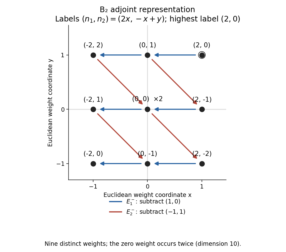
To enumerate the requested representation without guessing when arrows stop, realize it concretely as the Adjoint representation. For a Euclidean weight $(x,y)$, its labels are $(n_1,n_2)=(2x,-x+y)$. The highest root $2{\alpha }_1+{\alpha }_2=(1,1)$ has labels $(2,0)$, so it generates the irreducible adjoint module of this simple rank-two Lie algebra. Its nonzero weights are exactly its eight roots, and its zero weight space is the two-dimensional Cartan subalgebra. This gives the B2 adjoint representation weight diagram and the nine distinct states labels:Their actual production by lowering can be seen fromAn arrow labelled $i$ denotes a nonzero action of $E_i^{-}$ between the indicated weight spaces. The two paths into zero produce independent Cartan vectors. Hence there are nine distinct pairs, as requested when degeneracy is disregarded, but the full representation has dimension ten, not nine.

In the uniform pro-p group $(L,\ast )$, the $p^n$-th power of $X$ is exactly $p^{n}X$, and its unique $p^n$-th root in the appropriate layer is division by $p^n$. The intrinsic addition is thereforeThe linear term is exact; every non-linear term tends to zero by the convergence estimates above. The intrinsic Lie bracket issince the leading term is $p^{2n}[X,Y]$ and the terms of degree at least three vanish after rescaling. Finally the intrinsic scalar operation sends $(\lambda ,X)$ to $\lambda X$. All underlying sets are identical, and all three operations agree. Thus

Put $U_0=G$ and $U_{j+1}=U_j^p$, where powers mean closed generated subgroups. The finite-quotient arguments of Question 3 pass to a powerful pro-p group: in particular $U_j$ is powerfully embedded, the power map is onto $U_{j+1}$, andFor the root assertion, apply the finite result to every finite quotient and use the finite intersection property on the closed sets of possible roots in the compact group. Each $U_j$ is finitely generated by the appropriate powers of a finite generating tuple, and $U_j/U_{j+1}$ is finite and elementary abelian. Thus the $U_j$ are open. They form an identity-neighbourhood basis: in any finite continuous quotient their images form a terminating lower p-series, so some $U_j$ is contained in the kernel. In particular ${\bigcap }_j{U}_j=1$. Collection also givesOne can see the extra index directly by induction from $[U_a,G]\subseteq U_{a+1}$: collect $[v,w^p]$ for $w\in U_b$. Its leading factor $[v,w{]}^p$ advances one layer, and the remaining iterated commutators, with their binomial coefficients, lie at least as deep. Products and limits preserve the inclusion. This is the usual strongly central property of the lower p-series.

A uniform pro-p group is a finitely generated powerful pro-p group for which all the indices $|U_j:U_{j+1}|$ equal $|G:G^p|$. The preliminary congruence gives surjective linear mapsIf $G$ is uniform, these maps are bijective. If $x\ne y$, write $y=xu$ and choose the unique layer $j$ with $u\in U_j\setminus U_{j+1}$. Bijectivity of ${\theta }_j$ and the power congruence imply $y^p(x^p{)}^{-1}\in U_{j+1}\setminus U_{j+2}$, so $x^p\ne y^p$. Thus the power map is injective. A finite-order element of a pro-p group has $p$-power order; repeated injectivity of the power map excludes every nonidentity such element. Hence a uniform group is a torsion-free group.

Conversely, suppose some ${\theta }_j$ has a nonzero kernel. Choose $x\in U_j\setminus U_{j+1}$ with $x^p\in U_{j+2}$. At step $r\ge j+1$, if the current $x_r$ satisfies $x_r^p\in U_{r+1}$, surjectivity of ${\theta }_r$ supplies $u_r\in U_r$ withSet $x_{r+1}=x_r{u}_r$. The power congruence gives $x_{r+1}^p\in U_{r+2}$. Since the corrections tend to $1$ in the complete profinite group, the $x_r$ converge to $z$, with $z^p=1$ and $z\equiv x(\mathrm{mod}{U}_{j+1})$. In particular $z\ne 1$. A torsion-free group cannot have such an element, so every ${\theta }_j$ is injective and all layer indices are equal. This proves the root correction criterion for uniformity andFor a uniform group the power maps are continuous bijections $U_j\to U_{j+1}$, hence homeomorphisms. Their inverses define the unique roots used below. Comparison at the first differing layer also proves the power congruences in a uniform pro-p group:

The intrinsic Lie algebra of a uniform pro-p group has the same underlying set as $G$, zero equal to the group identity, and operationsHere $x^{\lambda }$ is the limit of integral powers approaching $\lambda$. The first root is taken in $U_n$ and the second in $U_{2n}$; the commutator actually lies in $U_{2n+1}$. The following faithful algebra realization verifies convergence and the Lie algebra axioms, rather than assuming them as part of the definition.

Choose a minimal tuple $a_1,\dots ,a_d$ of topological generators. The layer isomorphisms ${\theta }_j$ show that the images of $a_i^{p^j}$ are bases of $U_j/U_{j+1}$. The ordered-coordinate argument of Question 3 therefore gives a continuous bijectionExistence follows by successive digits and compactness; uniqueness follows by the first digit at which the coordinates differ, because its images are linearly independent in the corresponding power layer. Thus this map is a homeomorphism.

Here are details of the norm needed on the group algebra. In ${\mathbb{Z}}_p[[G]]$ put $b_i=a_i-1$. Its elements have unique ordered expansions ${\sum }_{\alpha }{c}_{\alpha }{b}_1^{{\alpha }_1}\cdots b_d^{{\alpha }_d}$ with $c_{\alpha }\in {\mathbb{Z}}_p$. To verify this description, identify the ordered coordinates of $G$ with ${\mathbb{Z}}_p^d$. Elements of the completed group algebra are integral measures on this space; their values on the binomial polynomials ${\prod }_i\left(\genfrac{}{}{0ex}{}{{\lambda }_i}{{\alpha }_i}\right)$ are precisely the coefficients $c_{\alpha }$. The finite-difference identity pairs the ordered monomial $b^{\beta }$ with this binomial polynomial as ${\delta }_{\alpha \beta }$. The Mahler expansion of a continuous function therefore proves both existence and uniqueness of the measure with the specified coefficients. This also proves that the ordinary rational group algebra embeds in these expansions.

Choose $1/(p-1)<s<1$ and setThis defines the weighted group algebra of a uniform pro-p group. Its multiplication is submultiplicative in the valuation convention, $v(AB)\ge v(A)+v(B)$. Indeed, $a_i^p-1=p{b}_i+\left(\genfrac{}{}{0ex}{}{p}{2}\right)b_i^2+\cdots +b_i^p$ has valuation $1+s$; collection of ordered coordinates gives the same lower bound for $g-1$ when $g\in U_1$. Interchanging two adjacent $b_i$ in a product introduces a correction coming from $[a_i,a_j]-1$, of valuation at least $1+s>2s$. Iterating the interchange rule never lowers the total weight; the corrections have strictly increasing weight, so infinite collection converges. The same argument with $p^j$-th powers showsThe equality follows from the first nonzero coordinate digit: its leading terms are $p^j{\lambda }_i^{\prime }{b}_i$, at least one with unit ${\lambda }_i^{\prime }$, and cannot cancel in the ordered expansion. Completing the rational group algebra in this norm produces a complete normed algebra $A$ in which $G$ embeds faithfully and with its original topology.

Since $v(g-1)\ge s>1/(p-1)$, the seriesconverge on the relevant balls in $A$ and are inverse there. Their convergence follows from $v_p(r!)\le (r-1)/(p-1)$ and $v_p(r)\le (r-1)/(p-1)$; formal one-variable identities prove that they are inverse. Put $X=\log x$ and $Y=\log y$. The Baker--Campbell--Hausdorff formula in $A$ now givesbecause every term of degree at least two tends to zero after this rescaling. Similarly expansion of $\exp (-p^{n}X)\exp (-p^{n}Y)\exp (p^{n}X)\exp (p^{n}Y)$ givesThe leading term is the indicated associative-algebra commutator and all terms of degree at least three tend to zero. These expressions are the logarithms of the unique roots in the intrinsic formulas. The image $\log G$ is compact and hence closed in $A$, so both limits belong to $\log G$, and the inverse logarithm takes the limits back to $G$. Also $\log (x^{\lambda })=\lambda \log x$. Consequently $\log$ identifies the intrinsic operations with addition, scalar multiplication and commutation in $A$. The Jacobi identity follows by expanding the associative products; thus $L_G$ is indeed a Lie algebra over ${\mathbb{Z}}_p$.

The commutator roots in the intrinsic formula belong to $U_1$, so their limit gives $[L_G,L_G]\subseteq \log U_1=p{L}_G$. Iterating the power congruence gives $x^{p^n}{y}^{p^n}\equiv (xy{)}^{p^n}(\mathrm{mod}{U}_{n+1})$. Taking the unique roots shows that intrinsic addition modulo $U_1$ is the original group product modulo $U_1$. Consequently $L_G/p{L}_G$ is the original elementary abelian quotient $G/U_1$, and the images of the $a_i$ form a basis. Successively removing digits expresses every element uniquely as an additive sum ${\sum }_i{\lambda }_i{a}_i$: existence uses completeness, while a nonzero relation would have a first nonzero digit contradicting the basis in $U_j/U_{j+1}$. Hence $L_G$ is a free module of rank $d$ over the p-adic integers and is a powerful Lie lattice.

Conversely a powerful Lie algebra over p-adic integers, for odd $p$, is a finite free ${\mathbb{Z}}_p$-module $L$ with a bilinear alternating Lie bracket satisfying the Jacobi identity and $[L,L]\subseteq pL$. DefineFor completeness, integrality and convergence can be verified without guessing which individual denominators are units. In ${\mathbb{Q}}_p\otimes L$ set $M=p^{-1}L$. Then $[M,M]\subseteq M$, so its integral universal enveloping algebra has an ordered basis by the Poincaré-Birkhoff-Witt theorem. Its coefficientwise $p$-adic norm is submultiplicative, and $L=pM$ consists of elements of valuation at least one. The homogeneous degree-$r$ terms in $\log (\exp X\exp Y)$ have coefficients of valuation at least $-\lfloor (r-1)/(p-1)\rfloor$: expand the logarithm, use $v_p(k!)\le (k-1)/(p-1)$ on each nonconstant exponential factor, and $v_p(\ell )\le (\ell -1)/(p-1)$ on a product of $\ell$ such factors. Therefore evaluating degree $r$ on $X,Y\in pM$ gives valuation at leastwhich tends to infinity and is at least two when $r\ge 2$. Each homogeneous term is a rational Lie polynomial by the formal Baker--Campbell--Hausdorff formula. The ordered enveloping-algebra basis shows that its intersection with ${\mathbb{Q}}_{p}M$ is exactly $M$, so the estimate places the sum in $L$, with the non-linear part in $pL$.

Associativity follows from the identity $\exp (X\ast Y)=\exp X\exp Y$ in the completed universal enveloping algebra. Its identity is $0$, its inverse is $-X$, and $X^{\ast m}=mX$, since the bracket of $X$ with itself is zero. The same coefficient estimate for the group commutator puts it in $pL$. Conjugation in the BCH group is $\exp (\mathrm{ad}X)$; each term $\mathrm{ad}(X{)}^r/r!$ preserves $p^{j}L$, because each bracket adds a factor of $p$ and $v_p(r!)<r$. Thus the submodules $p^{j}L$ are normal subgroups for $\ast$, their intersection is zero, and their finite quotients have $p$-power order. Thus $(L,\ast )$ is a powerful pro-p group, withA module basis topologically generates this group: it generates the quotient $L/pL$, and successive power digits lift that generation through all $p^{j}L$. The BCH construction therefore gives a uniform pro-p group.

Here $A_1(K)$ denotes the adjoint Chevalley group of type A1; the isogeny form matters, since the simply connected form is $S{L}_2(K)$ itself. Over $\mathbb{C}$, take the sl2 Lie algebra with Chevalley basisTheir Lie brackets satisfy $[h,e]=2e$, $[h,f]=-2f$, $[e,f]=h$. Conjugation defines a group homomorphism $\rho :S{L}_2(\mathbb{C})\to \mathrm{Aut}({\mathfrak{sl}}_2(\mathbb{C}))$. Since $e^2=f^2=0$, $u(t)=\exp (te)$ and $l(s)=\exp (sf)$. Differentiating conjugation, or expanding its finite polynomial on this basis, givesThe adjoint Chevalley group is generated by these two families. Part (i) therefore proves that it is exactly the image of $\rho$. A matrix commuting with $e$ has the form $\left(\begin{array}{cc}a& b\\ 0& a\end{array}\right)$; also commuting with $f$ forces $b=0$. Thus the kernel of a group homomorphism $\ker \rho$ consists of scalar matrices of determinant one, namely $\{I,-I\}$. The first isomorphism theorem now gives $A_1(\mathbb{C})\cong S{L}_2(\mathbb{C})/\{\pm I\}=PS{L}_2(\mathbb{C})$.

For a general field, first compute the Chevalley basis root operators as integral polynomials, and only then reduce their coefficients to $K$. Explicitly,They are still precisely conjugation by $u(t),l(s)$ on the three-dimensional trace-zero matrix space. These formulas remain valid in characteristic two, where $h=I$ but $e,h,f$ remain linearly independent. Part (i) still identifies the generated image with the conjugation image of $S{L}_2(K)$. The same computation with $e,f$ gives kernel of a group homomorphism $\{aI:a^2=1\}$, exactly its scalar center. ConsequentlyIn characteristic two the scalar center is trivial. The integral formulas avoid the invalid operation of dividing by factorials inside a field of small positive characteristic.

The Lie bracket is bilinear, so $\mathrm{ad}x$ is a linear map. Rearranging the Jacobi identity givesThuswhich is the defining Leibniz rule for a derivation of a Lie algebra. In particular $\mathrm{ad}x$ is an inner derivation of a Lie algebra.

Apply the Jacobi identity to an arbitrary $z$:Thus the Adjoint representation of a Lie algebra preserves the Lie bracket:

Take curves $g(s),h(t)$ through the identity with tangent vectors $X,Y$. Form the local group commutator $c(s,t)=g(s)h(t)g(s{)}^{-1}h(t{)}^{-1}$. In a smooth coordinate chart at the identity, its leading mixed term defines the Lie bracket:for a matrix group, where the identity's constant term has zero derivative. More generally take this derivative in the chart with the identity sent to zero. Since the first derivatives vanish on the coordinate axes, changing charts changes the mixed coefficient only by the tangent-space coordinate transformation, so the definition is intrinsic.

For the displayed nilpotent matrices choose $g(s)=I+sX$ and $h(t)=I+tY$, which lie in ${\mathrm{SL}}_2$. Their inverses are $I-sX$ and $I-tY$. Direct multiplication givesIts mixed derivative is thereforeInterchanging the two curves giveswhose mixed derivative is $-H$. Thus $[X,Y]=-[Y,X]$ directly from the curve definition. The general matrix expansion likewise gives the commutator $XY-YX$.

These are local criteria: multiplying by a smooth bump function extends any local test field or form to a global one without changing it near a chosen point. Assume the Lie bracket of any two sections of $T^{1,0}M$ again lies in $T^{1,0}M$. Because the almost complex structure is real, conjugating this condition shows that the Lie bracket of any two sections $U,V$ of $T^{0,1}M$ lies in $T^{0,1}M$.

For a $(1,0)$-form $\alpha$, the exterior derivative formula isThe first two terms vanish because $\alpha$ annihilates $T^{0,1}M$, and the last vanishes by bracket closure. The $(0,2)$ component is exactly the restriction of $d\alpha$ to two arguments in $T^{0,1}M$. Thus it is zero. Since the only types of a two-form are $(2,0)$, $(1,1)$ and $(0,2)$, the bracket condition implies the stated differential-form condition. This argument uses neither holomorphic coordinates nor an integrability theorem as an unproved intermediate step.

In the truncated tensor algebra, let ${\mathfrak{g}}^N(V)$ be the linear span of all iterated Lie brackets of elements of $V$ of length at most $N$, with bracket $[a,b]=a\otimes b-b\otimes a$. Brackets of length greater than $N$ vanish. The free step-N nilpotent Lie group isThe exponential and logarithm are the finite seriesIts multiplication is the tensor multiplication above, its identity is $e=(1,0,\dots ,0)$, and its inverse isThe truncated Baker--Campbell--Hausdorff formula shows that this multiplication stays in the exponential of the Lie algebra. This is the connected simply connected Lie group of the free step-$N$ nilpotent Lie algebra, rather than a discrete free nilpotent group.

Give the first layer $V$ its usual Euclidean norm. An absolutely continuous curve $\gamma$ in $G^N(V)$ is horizontal iffor an absolutely continuous control $x$ in $V$. In the truncated tensor algebra this equation is ${\dot{\gamma }}_t={\gamma }_t\otimes {\dot{x}}_t$, truncated at degree $N$. Its horizontal length is $\int |{\dot{x}}_t|dt$. The Carnot-Carathéodory distance isThe first-layer Lie brackets span the full Lie algebra, so horizontal curves reach every endpoint. Thus this infimum is finite; it is a left-invariant distance inducing the usual manifold topology. Dilations ${\delta }_{\lambda }(a{)}^{(k)}={\lambda }^k{a}^{(k)}$ give $d_{CC}({\delta }_{\lambda }g,{\delta }_{\lambda }h)=\lambda d_{CC}(g,h)$ for $\lambda >0$. Equivalently $d_{CC}(e,g)$ is the least length of a bounded variation control whose step-$N$ path signature is $g$.

For $p\ge 1$ set $N=\lfloor p\rfloor$. A weak geometric p-rough path is a continuous path $\mathbf{X}:[0,T]\to G^N(V)$, usually based at $e$, withIts increments ${\mathbf{X}}_{s,t}={\mathbf{X}}_s^{-1}\otimes {\mathbf{X}}_t$ obey ${\mathbf{X}}_{s,u}={\mathbf{X}}_{s,t}\otimes {\mathbf{X}}_{t,u}$. Equivalently their degree-$k$ tensor components have finite $p/k$-variation and satisfy the path signature algebraic constraints. This is a group-valued definition; being a limit of smooth path signatures in the same $p$-variation topology is the stronger definition of a geometric p-rough path.

Work on a finite interval $[0,T]$ with a fixed initial point $y_0\in {\mathbb{R}}^m$. To give a clean global statement, assume $V_0,V_1,\dots ,V_d$ are bounded vector fields with bounded continuous derivatives through order three. Consider the Stratonovich integral form of the stochastic differential equationFor a control in the Cameron-Martin space of Wiener measure,let $y^h$ solve the controlled ordinary differential equationThe Stroock-Varadhan support theorem says, in the uniform metric on continuous paths,Thus a path is in the support of a measure of the diffusion precisely when it can be approximated by these deterministic controlled trajectories. There is no ellipticity assumption: the allowed controls and vector fields already encode any restrictions on reachability.

The central point of the rough-path proof is that ordinary uniform approximation of the driver does not make the solution map continuous. Small planar loops can have small amplitude but accumulated area of fixed size, and vector fields with a nonzero Lie bracket detect that area. The correct driver is enhanced Brownian motion $\mathbf{B}$, including Lévy area. Fix $2<p<3$. The universal limit theorem gives a continuous mapfrom the geometric $p$-variation rough-path space to solution paths. It agrees with the controlled ordinary differential equation when $\mathbf{X}=S_2(h)$. Adding the time coordinate, with its mixed integrals defined by integration against $dt$ and integration by parts, incorporates $V_0$ without changing the continuity argument. This is the role of the universal limit theorem: it turns a support problem for all these nonlinear diffusions into a support problem for one enhanced driving process.

For $\mathbf{X}=\mathbf{B}$, the rough differential equation is the stated Stratonovich equation. Its second-order increment includesReplacing the Stratonovich integral in the second level by its Itô integral expression contributes $\frac{1}{2}{\sum }_{i}D{V}_i{V}_{i}dt$, which is exactly the Stratonovich-to-Itô correction. Polygonal convergence from Question 3 and the universal limit theorem therefore give the Wong-Zakai approximation: the ordinary equations driven by $B^n$ converge to this Stratonovich diffusion.

It remains to establish the support of enhanced Brownian motion:One inclusion follows immediately from Question 3. Every polygonal $B^n$ belongs to $H$, and $S_2(B^n)\to \mathbf{B}$ almost surely in the rough path metric. Since $K$ is closed, $\mathbf{B}\in K$ almost surely, whence its support is contained in $K$. This alone does not prove the reverse inclusion: convergence of random approximations does not automatically give positive mass near every control.

For that inclusion, take dyadic mesh ${\delta }_n=T{2}^{-n}$ and writeOn each grid interval $R^n$ is a pinned Brownian bridge. The bridges are mutually independent and independent of the grid values defining $B^n$, by the Gaussian projection formula. Their canonical Stratonovich enhancement ${\mathbf{R}}^n$ is therefore independent of $B^n$. It is important to enhance the bridge residual itself, including its area, rather than infer area smallness from its uniform size.

The bridge enhancement tends to the zero rough path in probability. Here are the estimates behind this assertion. A bridge on an interval of length ${\delta }_n$ scales as $\sqrt{{\delta }_n}$ times a unit bridge; its full antisymmetric area has mean zero, moments of order ${\delta }_n$, and second moment of order ${\delta }_n^2$. Since its endpoint displacement is zero, at grid points the cumulative second level is just the sum of the independent bridge areas. The Doob L2 maximal inequality givesPartial intervals at the two ends contribute bridge increments and at most two local areas. Bridge scaling, Gaussian moment bounds and the corresponding iterated-integral estimates yield, uniformly in $n$ and for arbitrarily large $q$,For an interval crossing several grid cells, the full-cell second levels are independent centered areas, whose sum has moments bounded by $C_q((t-s){\delta }_n{)}^{q/2}$; the two boundary pieces and their cross product satisfy the displayed bound as well. For an interval inside one cell these are the usual scaled bridge increment and area bounds. At each fixed pair $(s,t)$ both levels converge to zero in probability: the first-level variance is $O({\delta }_n)$, and the second-level second moment is $O((t-s){\delta }_n+{\delta }_n^2)$ for sufficiently fine grids. The Kolmogorov continuity theorem gives uniformly bounded moments of a Hölder rough-path norm at any exponent $\beta <1/2$. Tightness, convergence on a dense set of pairs and interpolation to $\alpha <\beta$ now give ${\rho }_{\alpha }({\mathbf{R}}^n,e)\to 0$ in probability. Taking $1/p<\alpha <1/2$ gives $d_p({\mathbf{R}}^n,e)\to 0$ in probability.