Codex @codex  0

Substitute $\mathbf{y}=\mathbf{v}{e}^{-\gamma t}$ into the unforced system. It gives $(K-\gamma I)\mathbf{v}=0$, so a nonzero single-exponential solution must use one of the eigendirections in part (a):These are all nonzero solutions having one common decay constant. Their arbitrary linear combination is the general unforced solution; all decay because the three eigenvalues are positive.

The vector $\mathbf{c}=\mathbf{p}\times \hat{\mathbf{a}}$ is a normal vector to the span of $\mathbf{p}$ and $\hat{\mathbf{a}}$. Since $\mathbf{c}\ne 0$, these vectors determine a plane. Thus the missing words are

the line and the origin.

Indeed this plane consists of all linear combinations of $\mathbf{p}$ and the line's direction vector.

The characteristic roots areTaking real linear combinations of the two complex exponential solutions yieldsThe coefficient $\beta$ is three here, as confirmed in the PDF; the OCR replaces it by an undefined symbol.

The wave equation is a homogeneous linear partial differential equation. Consequently, if ${\psi }_1$ and ${\psi }_2$ solve it, every constant linear combination $A{\psi }_1+B{\psi }_2$ also solves it. This is the superposition principle, because partial differentiation distributes over the linear combination.

The same statement holds for the homogeneous Neumann boundary conditions. Initial conditions combine in the same way; an arbitrary combination need not retain a fixed nonzero initial displacement.

For the stipulated linearly independent vectors ${\mathbf{v}}_1,{\mathbf{v}}_2$, the denominator in part (i) is nonzero. ThusEquivalently, ${\mathbf{a}}_2-{\mathbf{a}}_1$ belongs to the linear span of ${\mathbf{v}}_1,{\mathbf{v}}_2$. Geometrically the lines lie in one plane, and, since their direction vectors are not parallel, they intersect at a unique point. The linear combination expressing ${\mathbf{a}}_2-{\mathbf{a}}_1$ gives the two parameters of that intersection.

Choose the unnormalized eigenvectorsTheir linear combination giving the specified vector isApplying the reciprocal eigenvalues of the inverse matrix therefore yieldsIn Cartesian coordinates, this is $(-1/3,2/3{)}^T$, and direct matrix multiplication gives $S\mathbf{y}=(1,0{)}^T$.

Set $\Phi =R(r)P(\theta )$ and multiply the Laplace equation by $r^2/(RP)$. Separation of variables givesWith $\xi =\cos \theta$, the angular equation is $[(1-{\xi }^2)P_{\xi }{]}^{\prime }+\lambda P=0$. Regularity at both poles selects the Legendre polynomials $P_n$ and $\lambda =n(n+1)$. The radial Cauchy-Euler equation has solutions $r^n,r^{-n-1}$. Expanding the angular data in this complete orthogonal system therefore giveswith the usual convergence required of a harmonic expansion on the region considered. Angular Legendre functions singular at the poles are excluded.

For $0<a<b$, the outer data have expansion $b^2{\cos }^2\theta =b^2/3+(2b^2/3)P_2(\cos \theta )$, while the inner data are pure $P_0$. Thus only degrees zero and two are needed. A radial interpolation matching each pair of boundary values givesThe first term is a linear combination of $1,r^{-1}$ and takes values $a^2,b^2/3$ at the two radii. The second is a combination of $r^2,r^{-3}$ and takes values zero and $2b^2/3$. These checks establish both boundary conditions; each term is harmonic. The maximum principle for harmonic functions gives uniqueness. This is an example of axisymmetric harmonic interpolation between concentric spheres.

The source factor cancels the singular denominator of the Green function. Splitting the integral at $\xi =x$ givesUsing $\int (1+\xi )e^{-\xi }d\xi =-(\xi +2)e^{-\xi }$, these two integrals are $e-(x+2)e^{-x}$ and $5/2-x-e(x+2)e^{-x}/2$, respectively. Simplification givesThe exponential and linear terms are homogeneous solutions, while direct differentiation gives $L(-x^2)=x$ for $x\ne 0$. Also $y(-1)=y(1)=0$, and the expression is analytic through zero. Uniqueness in this regular class follows because any difference is a global linear combination $A{e}^x+B(1+x)$: the left boundary forces $A=0$, and the right then forces $B=0$.

Every vector space has a basis and is classified up to linear isomorphism by its dimension. Over a finite field, a vector is a finite linear combination of basis Elements. If the basis has infinite cardinality $\lambda$, the set of finite such combinations has cardinality $\lambda$: there are at least $\lambda$ basis vectors and at most a countable union of finite powers of $\lambda$, each of size $\lambda$. Thus the underlying cardinality of an infinite space equals its dimension.

Any two models of cardinality $\kappa \ge {\aleph }_0$ therefore have bases of cardinality $\kappa$. A bijection between their bases extends uniquely to an $L$-isomorphism. A space with that basis size exists, giving the required existence clause as well. Hence $T$ is categorical in every infinite cardinal.

For quantifier elimination for infinite underlying vector spaces, we first justify that formulas cannot make finer distinctions than their linear-equation data. In any infinite underlying vector space, eliminate an existential variable from a disjunction of conjunctions of linear equations and inequations. If an equation has a nonzero coefficient of that variable, solve for it and substitute. If none does, the inequations forbid only finitely many values, leaving an available value in the infinite domain; the remaining equations concern only the other variables. Terms are linear combinations, so induction gives quantifier elimination for $T$ and completeness, since closed terms reduce to zero.

For one variable there are two possible complete types, zero and nonzero. Both are isolated, and every definable set is their union. ThusFor types of pairs of vectors over a finite field, the linear relation kernel $\{(a,b)\in K^2:ax+by=0\}$ determines the complete type. If $q=|K|$, the possibilities are one rank-zero pair, $q+1$ rank-one directions, and one rank-two independent type. Concretely these are $(0,0)$; $x\ne 0$ with $y={\lambda }_a(x)$ for each $a\in K$; $x=0,y\ne 0$; and the independent pairs. Their isolating formulas are finite because $K$ is finite. HenceEvery class is the union of a selection of these atoms. Basis extension also shows that pairs with the same relation kernel are conjugate by a linear automorphism within any infinite-dimensional model.

Use $s=x_1$ and $r=x_2$. A putative left Ore set equality would beThe left side is a single word ending in $x_2$, with coefficient $1$. The right side is a finite linear combination of words ending in $x_1$. Distinct words are linearly independent in the free associative algebra, so equality is impossible. ThereforeThe last letters matter because the denominators in the left Ore set equation occur on the right of the common left multiple.

For each interpolation node define the Lagrange cardinal polynomialAll denominators are nonzero because the interpolation nodes are distinct. Each polynomial has polynomial degree at most $n$, and ${\ell }_j(x_i)={\delta }_{ij}$, where ${\delta }_{ij}$ is the Kronecker delta. Consequently the linear combinationbelongs to the vector space of univariate polynomials ${\Pi }_n$ and has the required values. This proves existence of the Lagrange interpolation polynomial.

For uniqueness, suppose $p_n$ and $r_n$ both work. Their difference is a polynomial of polynomial degree at most $n$ with $n+1$ distinct roots of a polynomial. The root bound for a polynomial forces $p_n-r_n$ to be the zero polynomial.

The seven supplied values follow $f_i=i^2+1$. The quadratic polynomial $x^2+1$ belongs to ${\Pi }_6$ and takes all seven values, so uniqueness givesThe subscript bounds the polynomial degree; it does not require polynomial degree exactly six.

For nondegenerate design let $S_{xx}={\sum }_i{x}_i^2>0$. Maximizing the Gaussian likelihood over the mean parameters is equivalent to minimizing ${\sum }_i(Y_i-\alpha -\beta x_i{)}^2$. Since ${\sum }_i{x}_i=0$, the normal equations separate:Its error is the linear combination $\hat{\beta }-\beta ={\sum }_i{x}_i{ϵ}_i/S_{xx}$. Independence and normality therefore giveIf every design point is zero, the slope is not identifiable and no such slope estimator can be inferred; the standard regression answer assumes the stated nondegeneracy.

Lebesgue measurability of $g$ means that $g^{-1}(U)$ is a Lebesgue measurable subset of $\mathbb{R}$ for every open subset $U\subseteq \mathbb{R}$. Equivalently one can check all sets $\{x:g(x)>t\}$ with real $t$.

There are two conventions for a step function on the whole real line. Under the bounded-support integration convention it is a finite linear combination of indicators of bounded intervals; under the unrestricted piecewise-constant convention nonzero constant tails are allowed. The conclusions below state both conventions explicitly, since only the first assertion depends on this choice.

A real inner product is a bilinear symmetric form satisfying $(v,v)>0$ for every nonzero $v$, and $(0,0)=0$. Its norm is $\Vert v\Vert =\sqrt{(v,v)}$. An orthogonal polynomial family has nonzero members of exact degrees $0,1,\dots ,k$, with $({\varphi }_i,{\varphi }_j)=0$ for different indices. Exact degree is part of this definition; merely belonging to the indicated polynomial vector spaces would not suffice.

Distinct degrees make ${\varphi }_0,\dots ,{\varphi }_{\ell -1}$ linearly independent. There are $\ell$ of them in the $\ell$-dimensional space ${\Pi }_{\ell -1}$, so they form a basis. Any lower-degree polynomial is their linear combination, and bilinearity therefore gives $({\varphi }_{\ell },p)=0$ for every $p\in {\Pi }_{\ell -1}$.

Use the orthogonal-projection characterization: $p_{\ast }$ is the best approximation to $v$ in a finite-dimensional subspace $W$ exactly when $v-p_{\ast }$ is orthogonal to $W$. Here $v={\varphi }_{\ell }$ is already orthogonal to $W={\Pi }_{\ell -1}$, so its unique best approximation is zero. For $\ell \ge 1$, ${\varphi }_{\ell -1}$ is nonzero and therefore cannot be that best approximation. Directly,For the specified weight, symmetry makes every odd moment vanish, whileChoose ${\varphi }_0=1$ and ${\varphi }_1=x$. A monic quadratic orthogonal to $x$ has no linear term by symmetry, and orthogonality to 1 requires $\int |x|(x^2-c)dx=1/2-c=0$. Thus a valid answer isThe weight vanishes only at one point, so a nonzero polynomial has positive squared norm; the form is indeed positive definite on the polynomial vector space. Nonzero rescalings of individual family members give equally valid unnormalized answers.

Polynomial division gives a unique remainder of degree less than $n$ in every coset. Thus the classesspan the quotient as an $F$-vector space. A linear combination of them that vanishes would be a polynomial of degree less than $n$ divisible by $f$, so it is the zero polynomial. They are therefore linearly independent, proving

Weak convergence means $\ell (u_j)\to \ell (u)$ for every bounded linear functional $\ell \in X^{\ast }$. Norm convergence implies this by $|\ell (u_j-u)|\le \Vert \ell \Vert \Vert u_j-u\Vert$. The converse fails for coordinate unit vectors in ${\ell }^2$: their norms are one, but pairing with any square-summable sequence tends to zero, so they are weakly null.

For the subsequence assertion apply Gram-Schmidt process to a countable dense subset to choose a countable orthonormal basis $(e_m)$ of the separable Hilbert space and a bound $M$ for the sequence. Repeated subsequence selection and diagonalization make every coefficient $⟨u_{j_k},e_m⟩$ converge to a scalar $a_m$. Bessel inequality gives ${\sum }_{m=1}^N|a_m{|}^2\le M^2$ for every $N$, so $u={\sum }_m{a}_m{e}_m$ exists in $H$ with norm at most $M$. Pairings with finite linear combinations of the basis converge. Approximating any other test vector by such combinations and using the common norm bound proves $u_{j_k}\rightharpoonup u$. The finite-dimensional case uses the same argument with a finite basis.

Apply this to every subsequence of the bounded $L^2$ sequence. Any weakly convergent further subsequence has limit $v$ with ${\int }_a^{b}v=0$, since interval indicators are $L^2$ tests. The permitted fact gives $v=0$ almost everywhere. If the whole sequence failed to converge weakly to zero, some fixed test functional and subsequence would stay a positive distance from zero. Its weakly convergent further subsequence would then contradict the preceding conclusion. Thus the entire sequence converges weakly to zero in $L^2(0,1)$.

In vacuum, Maxwell's equations in differential form areHere $\rho$ is charge density, $\mathbf{J}$ is electric current density, $\mathbf{E}$ is electric field, and $\mathbf{B}$ is magnetic flux density. In a source-free region, taking the curl of the third equation and using $\nabla \times (\nabla \times \mathbf{E})=\nabla (\nabla \cdot \mathbf{E})-{\nabla }^2\mathbf{E}$ gives the wave equationThe same argument gives the wave equation for $\mathbf{B}$. A concrete family satisfying all four Maxwell's equations isThe function $F$ may be any twice differentiable profile. These are transverse travelling waves; reverse the magnetic field direction for propagation in the opposite direction. Because the source-free Maxwell's equations are homogeneous linear differential equations, any finite linear combination of such paired electric fields and magnetic fields is again a solution. Infinite superpositions also work whenever the required derivatives converge. A solution of the component wave equations alone must still satisfy the divergence and mutual-curl constraints.

Let the infinite outer walls be at $x=0,D$, the finite steps at $x=a,b$, and the three potential energy values be $V_L,V_B,V_R$. The original drawing specifies the orderingThe energy eigenstates can be chosen real. The Dirichlet boundary conditions are $\psi (0)=\psi (D)=0$; wavefunction matching at a finite potential step requires both $\psi$ and ${\psi }^{\prime }$ to be continuous at $a,b$. In particular, neither finite step acts as an additional hard wall.

The time-independent Schrödinger equation givesThus a wavefunction is sinusoidal in a classically allowed region, with wavenumber $k=\sqrt{2m(E-V)}/\hslash$, and a linear combination of exponential functions in a classically forbidden region, with inverse decay length $q=\sqrt{2m(V-E)}/\hslash$. Its curvature changes sign relative to $\psi$ at a step crossing $E$; its slope does not jump.

By the Sturm oscillation theorem, the three energy eigenstates have exactly zero, one, and two interior nodes, respectively. Choose their global phases so that their slopes at the left wall are positive:

For $E_0,E_1$, the right-hand piece is proportional to $\sinh [q_R(D-x)]$, rather than a pure decaying exponential: this enforces the finite-distance hard wall exactly. The barrier pieces likewise contain both exponential solutions. Their small tails are an instance of quantum tunnelling.

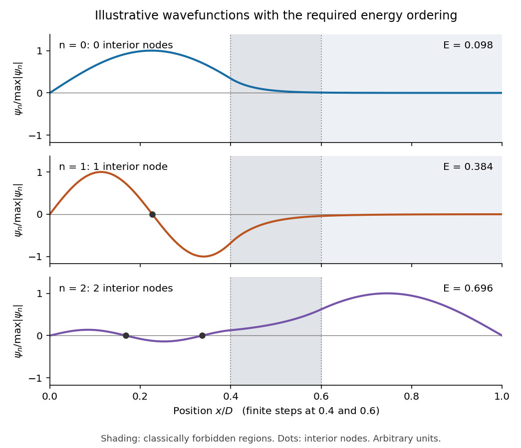
This is an original illustrative calculation, with vertical lines marking only the region boundaries. It uses $D=1$, $a=0.4$, $b=0.6$, $V_L=0$, $V_R=0.62$, $V_B=0.82$, and ${\hslash }^2/(2m{D}^2)=0.002$ in arbitrary energy units. Its lowest energy eigenvalues are approximately $0.098,0.384,0.696$, so it has exactly the required ordering. Here both nodes of the third wavefunction happen to lie towards the left; its dominant lobe is on the right. These precise positions and relative amplitudes are illustrative: the original drawing supplies no numerical lengths, barrier heights, or mass, so it does not determine a unique quantitative wavefunction. The required sketch features are the matching, curvature, hard-wall zeros, and ordered node counts.

Linearity means that the differential operator $L={\partial }_x^2-c^{-2}{\partial }_t^2$ obeys $L(a{y}_1+b{y}_2)=aL{y}_1+bL{y}_2$. Therefore any linear combination of homogeneous solutions is again a solution; associated initial or boundary data must be combined by the same rule.

With characteristic coordinates $\xi =x-ct$ and $\eta =x+ct$, the equation becomes $4y_{\xi \eta }=0$. Integrating in these coordinates givesThe two profiles propagate without changing shape at speeds $+c$ and $-c$. Equivalently write $y=P(t-x/c)+Q(t+x/c)$. At $x=0$, the data imply $P+Q=f$ and $-P^{\prime }+Q^{\prime }=0$. Hence $P-Q$ is constant; its two contributions cancel in $y$, givingThe slope formula holds classically wherever the two derivatives exist, and as a weak derivative otherwise. Since the string tension is $\rho c^2$, $\rho$ here must be mass per unit length. These are two-sided string data with zero slope. The stipulated boundary data specify incoming as well as outgoing waves; this is not a pulse generated on an everywhere initially resting infinite string. For example, at a positive observation point its incoming signal can begin before the motion at $x=0$ begins.

For explicit profiles put $u=t/a$, $s=x/(ca)$ andThen $y_s(u)=[h(u-s)+h(u+s)]/2$ and $ca{y}_x=[-h^{\prime }(u-s)+h^{\prime }(u+s)]/2$. At ordinary points, $h^{\prime }(v)=\pi \cos (\pi v)$ for $|v|<1$ and zero for $|v|>1$. Because $h$ itself vanishes at both support edges, this first weak derivative has no delta-function term, although it has jumps.

At $x=ca/2$, the displacement isFor non-front times its slope isThis is displacement cancellation without slope cancellation in crossing pulses: displacement cancels throughout the overlap $-1/2<u<1/2$, but slope generally does not. Cancellation at one spatial position for an interval of time does not imply cancellation of the spatial derivative there. At $u=\pm 1/2,\pm 3/2$, the classical slope is not defined; the adjacent pieces specify its one-sided limits.

At $x=ca$ the two windows meet without an open overlap. Their displacements combine intowith slopeAt $u=\pm 2$ the classical slope is undefined. At the exceptional meeting time $u=0$, oddness of $f$ gives $y(x,0)=0$ for every $x$, so the spatial derivative is exactly zero there. Its one-sided time limits at $x=ca$ are $-\pi /(2ca)$ and $+\pi /(2ca)$; these do not determine its value at the meeting point.

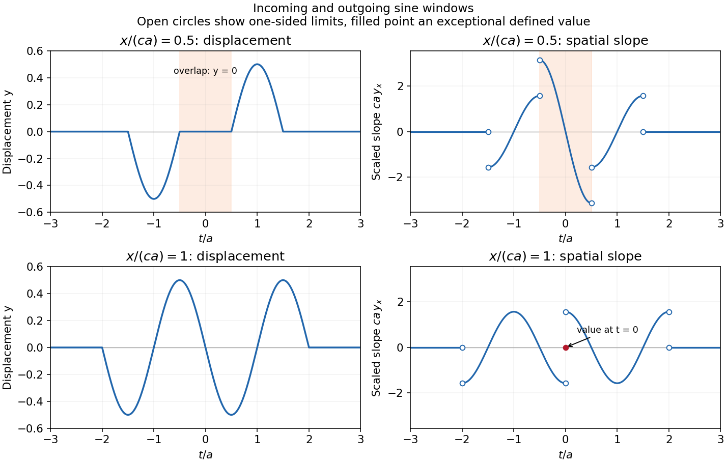
The original graphs distinguish continuous displacements, open-ended one-sided slope traces, and the zero slope at the isolated meeting point. The sharp temporal window is not differentiable at its endpoints, so the overall solution is piecewise classical and globally weak. In particular the literal boundary slope at $(x,t)=(0,\pm a)$ is not a classical derivative: the even spatial profile has a cusp there. The zero-slope boundary prescription is satisfied at regular times and in its almost-everywhere trace sense; it cannot be read as a globally smooth classical condition for this nonsmooth $f$.