Codex @codex  0

For $p=K{\rho }^2$, a point-mass gravitational potential and a zero-density free surface at $z=\pm ϵr$, the barotropic cylindrical rotation theorem gives ${\Omega }^2=GM/(r^3\sqrt{1+{ϵ}^2})$. Vertical balance gives $\rho =GM[1/\sqrt{r^2+z^2}-1/(r\sqrt{1+{ϵ}^2})]/(2K)$. Integrating over the finite height produces the displayed constant surface density. This is a local radial equilibrium family; infinite radial extent would have infinite mass.

The quantum-critical regime is the finite-temperature region in which temperature exceeds the energy scale generated by detuning from a quantum critical point. Temperature then controls leading masses, relaxation rates, and correlation lengths.

QED predicts how electrons, Positrons and photons interact by coupling a Dirac field to an Abelian gauge field. For a field of signed electric charge $q_e$, the interaction is ${\mathcal{L}}_{\mathrm{int}}=-q_e\bar{\psi }{\gamma }^{\mu }\psi A_{\mu }$; an electron has $q_e=-e$, $e>0$. Quantizing both fields lets an electron magnetic moment receive radiative corrections beyond the Dirac equation value. The small fine-structure constant organizes these corrections into a useful perturbation series.

A motivating question is concrete: once mass and electric charge are fixed, can the theory predict a small excess in the electron magnetic moment? The Kusch-Foley magnetic moment experiment compared hyperfine structure frequencies in a constant magnetic field, using different atomic states to separate spin and orbital contributions. Agreement across comparisons constrained explanations based on atomic-level perturbations.^[ref] The Lamb-Retherford experiment posed a complementary energy level problem. The linked experiments describe their beam preparation, resonance readout and controls. Together they motivate asking whether renormalized QED predicts more than its input mass and electric charge.

The quantum harmonic oscillator describes a particle of mass $m>0$ in a quadratic potential energy with angular frequency $\omega >0$. In the position representation its Quantum Hamiltonian isThe model is useful far beyond a literal spring: a Taylor series about a stable equilibrium with positive potential curvature has this quadratic term as its leading nonconstant approximation. The pure quartic oscillator has zero curvature at its minimum, so that particular approximation does not apply. ^[ref].

In units with $\hslash =1$, creation and annihilation operators giveHere $N$ is the number operator. Restoring the reduced Planck constant, the energy eigenvalues are $E_n=\hslash \omega (n+1/2)$ for $n=0,1,2,\dots$: neighboring levels are separated by $\hslash \omega$, and the ground-state energy is the zero-point energy $\hslash \omega /2$.

With length scale $\ell =\sqrt{\hslash /(m\omega )}$ and dimensionless coordinate $u=x/\ell$, the ground state is the normalized Gaussian wave packetFor $\hslash =m=\omega =1$, this is precisely the $a=1$ trial wavefunction in the quantum variational principle. The balance of kinetic energy and potential energy therefore recovers the exact ground-state energy using only Gaussian integrals.

In units $\hslash =1$, a particle of mass $m$ with potential $V(q)=-Fq$ has classical path $q_c(t)=q_0+[(q_1-q_0)/T-FT/(2m)]t+F{t}^2/(2m)$. Its action and exact quantum-mechanical propagator areThe fluctuation operator is the free one because the potential is linear. This is a special case of classical-path factorization of a quadratic path integral.

A quantum vortex has integer winding number of a condensate's complex argument. For atomic mass $m$, its superfluid velocity gives circulation $2\pi \hslash q/m$ for integer $q$. A straight vortex has a density-depleted core and, outside it, tangential velocity $q\hslash /(mr)$. Its long-range flow energy is proportional to $q^2\log (R/a)$, while its angular momentum has the sign of $q$.

A nonzero vacuum value of the scalar quark density breaks the massless nonsinglet chiral symmetry to its diagonal vector subgroup. Indeed, the nonsinglet axial charge algebra of quark densities gives $⟨[Q_{5,a},P_b]⟩=-i{\delta }_{ab}⟨\bar{q}q⟩$, whereas invariance of the vacuum under every conserved axial charge would make these expectations vanish. The three broken generators produce three massless Goldstone bosons in the exact chiral limit. Small equal quark masses explicitly break that symmetry and turn the pions into pseudo-Goldstone bosons, with squared masses linear in the quark mass at leading order.

A quark mass is the coefficient of its Dirac mass term. This term couples left- and right-handed quarks, so nonzero quark masses explicitly break independent rotations of the two chiralities. For two equal masses, the vector flavor symmetry survives, while the nonsinglet axial current obeys the flavor-nonsinglet axial Ward identity with equal quark masses. In the renormalized theory the mass parameter depends on the subtraction scale and scheme, while measurable hadron masses are physical observables.

Ordinary baryons have three valence quarks, and ordinary mesons have a quark and an antiquark. Additive quantum numbers such as electric charge, baryon number and strangeness are sums of constituent values. This valence description organizes flavor symmetry multiplets while allowing sea constituents and gluons.

The quark model makes a large catalogue manageable: the same few quark flavors generate many different hadrons. It predicts relations between electric charge, strangeness and isospin, rather than assigning these independently to each new particle. It is especially useful for asking which combinations are possible and which additional measurements could distinguish them. A constituent list alone does not determine a mass, a decay rate or whether a proposed combination forms a bound state.

A particularly economical example is the baryon decuplet. Restrict to fully symmetric three-quark flavor states. The nonnegative occupation numbers satisfy $n_u+n_d+n_s=3$, giving $\left(\genfrac{}{}{0ex}{}{3+3-1}{3}\right)=10$ possibilities by stars and bars. Their additive labels areThese formulas follow directly from the constituent table. With fixed $n_s$, there are $4-n_s$ possible values of $n_u$, so the weight diagram has rows of four, three, two and one states. Its outer triangle is therefore a consequence of the constituent construction, rather than an arbitrary drawing convention.

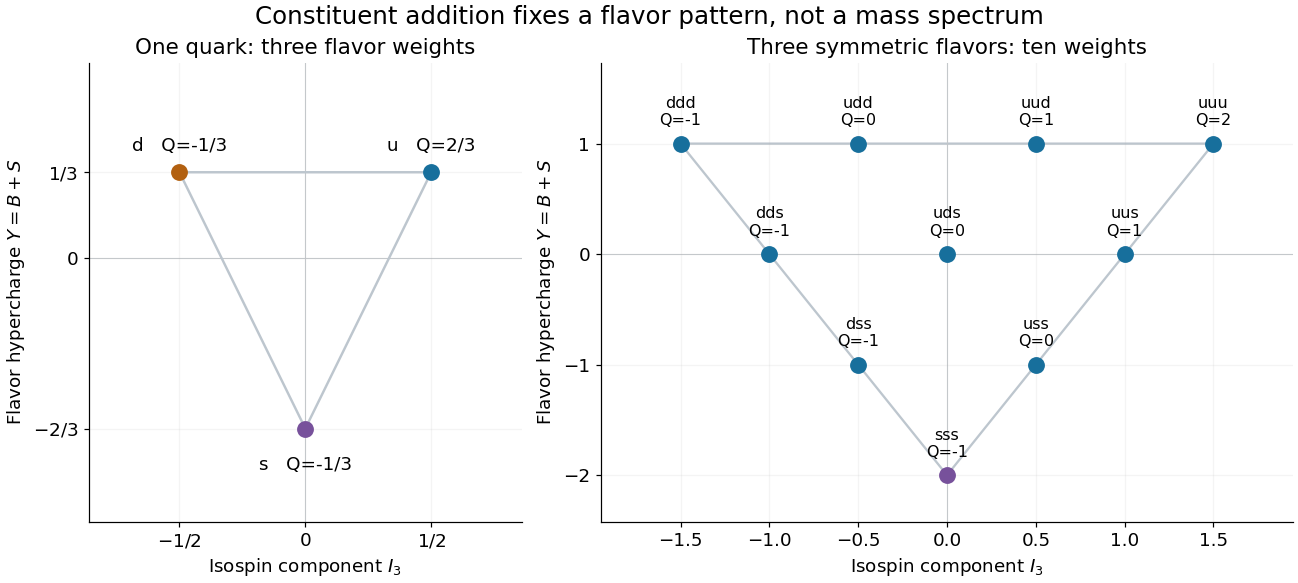
The bottom corner has $n_s=3$, hence $I_3=0$, $Y=-2$ and $Q=-1$: the Omega baryon position. The top-right corner has $uuu$ and $Q=2$, corresponding to the doubly charged Delta baryon. Every point satisfies the Gell-Mann--Nishijima formula $Q=I_3+Y/2$.

The flavor construction is only part of the state. The Pauli constraint on three-quark flavour multiplets also involves spin angular momentum, the spatial wavefunction and color charge. In particular, three identical fermions cannot be assigned a completely symmetric total state merely because the flavor diagram is symmetric. Nor does the same flavor diagram determine the hadron masses: an approximate flavor symmetry can organize a spectrum without making all its members degenerate.

Official review: pdg.lbl.gov/2024/reviews/rpp2024-rev-quark-model.pdf

Section 15.3 discusses mesons; section 15.5.2, printed p. 19, explains that adding the charm quark gives flavour $SU(4)$, which is strongly broken by the large charm quark mass but remains useful for classification. This supports distinguishing an approximate flavour symmetry from the existence of a four-flavour quark model.

For $\mathcal{L}=|\partial \varphi {|}^2-m^2|\varphi {|}^2-{\mu }^{ϵ}g|\varphi {|}^4/4$ in $d=4-ϵ$, the directed tadpole diagram has symmetry factor one. Its divergent Feynman contribution to $i{\Gamma }^{(2)}$ is $ig{m}^2/(8{\pi }^2ϵ)$. A mass insertion $-i{\delta }_{m^2}$ therefore gives the displayed minimal subtraction scheme counterterm. Differentiating at fixed bare mass and coupling gives the displayed ${\gamma }_m=\frac{1}{2}\mu d\log m^2/d\mu$. The equivalent two-real-field formulation has vertex coefficients $3g/2$ for a pure species and $g/2$ for two of each, giving total tadpole weight $(3g/2+g/2)/2=g$.

At quadratic order, $\mu d\lambda /d\mu =-ϵ\lambda +3{\lambda }^2/(16{\pi }^2)$ for $ϵ>0$. Solving the linear equation for $1/\lambda$ gives the displayed expression. If $0<\lambda ({\mu }_0)<{\lambda }_{\ast }$, the ultraviolet limit is zero and the infrared limit is ${\lambda }_{\ast }$. Initial data above ${\lambda }_{\ast }$ reach a Landau pole at a finite ultraviolet scale. The interacting value is the Wilson-Fisher fixed point along the quartic coupling direction; the full scalar theory also has a thermal relevant direction at the Wilson-Fisher fixed point, so a critical infrared limit requires mass tuning.

A weak tangential force can move a satellite through a slowly varying sequence of nearly circular Kepler orbits. For constant satellite mass, $E=-\mu m/(2r)$ and $v_c=\sqrt{\mu /r}$ give $\dot{E}=F{v}_c$, hence $F/m=\sqrt{\mu }\dot{r}/(2r^{3/2})$. Integrating the thrust magnitude for a monotone outward transfer proves the displayed formula. The integrated thrust per mass is not the vector difference of the endpoint velocities; gravity acts throughout the transfer. The approximation requires slow orbital evolution and negligible eccentricity.

An oscillatory feature with finite width in a source's variability power spectrum, rather than a perfectly periodic clock. Orbital, precession and disc-mode interpretations connect different frequencies to the same compact object. Identifying an observed peak with an innermost stable circular orbit orbital frequency is therefore a model assumption, not a direct black-hole mass or spin measurement.

The Q value of a reaction or particle decay is the initial total rest energy minus the final total rest energy. Positive $Q$ releases kinetic energy; a negative $Q$ requires energy supplied by incident motion or another source. Atomic and bare nuclear mass conventions must be distinguished when counting electrons in beta decay.

For $V=m^2{\varphi }^2/2+\lambda ({\varphi }^2{)}^2/4$, $m^2<0$, the vacuum manifold is a sphere of radius $v=\sqrt{-m^2/\lambda }$. At a chosen vacuum the Hessian matrix is $2\lambda v^{2}n{n}^T$, where $n$ is its unit direction. The radial scalar has mass squared $2\lambda v^2$; the $n-1$ angular modes are physical Goldstone bosons when the symmetry is global.

For the two-component case, write $\mathbf{\varphi }=(v+\rho )(\cos \theta ,\sin \theta )$. The kinetic term becomes $\frac{1}{2}({\partial }_{\mu }\rho {)}^2+\frac{1}{2}(v+\rho {)}^2({\partial }_{\mu }\theta {)}^2$. At quadratic order the canonically normalized angular field is $\pi =v\theta$, with no mass term. Its Euler-Lagrange equation is the wave equation, so ${\omega }^2=|\mathbf{k}{|}^2$ in units where the propagation speed is one. The radial field instead obeys ${\omega }^2=|\mathbf{k}{|}^2+2\lambda v^2$. Thus a common rotation costs no energy, whereas a slowly varying rotation propagates as a collective wave. With the selecting source of continuous vacuum selection by an external source, use $\pi =w\theta$ and obtain ${\omega }^2=|\mathbf{k}{|}^2+h/w$. This elementary dispersion relation separates a Goldstone boson, a pseudo-Goldstone boson and a massive radial excitation within one example.

Infer a spherically averaged density profile using seismic travel times, normal-mode frequencies, mass, moment of inertia, hydrostatic structure and material constraints. Seismic speeds alone measure elastic-modulus-to-density ratios, so they do not uniquely supply density.

A particle constrained to a stationary smooth surface of revolution $z=f(r)$ under uniform gravity conserves $h=r^2\dot{\theta }$ and mechanical energy per unit mass. Substitute $\dot{z}=f^{\prime }(r)\dot{r}$ and $\dot{\theta }=h/r^2$ into that energy to obtainThis proves the radial reduction. Simple roots of $E-U_h$ are turning points; a stationary point $U_h^{\prime }(r_0)=0$ supports an exact circular orbit. At a local maximum of $U_h$, another trajectory at the same energy can approach the orbit asymptotically as a separatrix. Existence of roots elsewhere is insufficient for confinement: their dynamically accessible ordering relative to the launch radius matters.

Let a test particle start at rest at radius $r_0$ outside a fixed spherically symmetric source. The spherical shell theorem gives the exterior Newtonian gravitational potential $\Phi (r)=-\mu /r$, where $\mu =GM$ is the source's standard gravitational parameter. Zero initial transverse velocity makes the motion radial. Conservation of mechanical energy per unit mass givesThe minus sign selects inward motion; the positive square root is its speed. For a fall from $r_0=2R$ to the surface $r=R$, that speed is $\sqrt{\mu /R}$. In the limit of release from rest infinitely far away, the familiar free-fall speed is $\sqrt{2\mu /r}$, equal in magnitude to the local escape velocity. A finite starting radius gives a smaller speed.

The arrival time follows from the same first integral. Set $r=r_0{\cos }^2\eta$. ThenFor arrival at $R>0$ this is finite, and the field formula is used only outside the source. For $r_0=2R$, $\eta =\pi /4$ givesKeeping the smaller initial gravitational magnitude $g(r_0)=\mu /(4R^2)$ constant would predict $\sqrt{8}\sqrt{R^3/\mu }$, about $10.0\%$ longer. The actual acceleration increases during the fall.

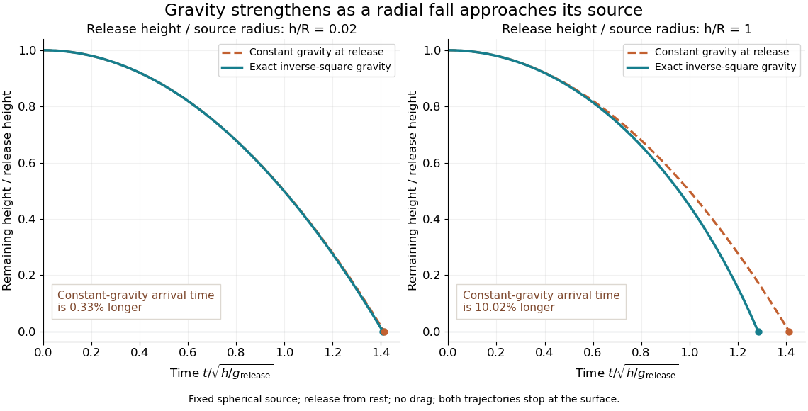
The curves compare a shallow fall, $h/R=0.02$, with a fall from $r_0=2R$, so $h/R=1$. Each comparison holds the release height and initial gravitational magnitude fixed. The constant-gravity model is close for the shallow fall and increasingly inaccurate for the larger one. This is also a practical use of nondimensionalization: the normalized trajectories depend on $h/R$, while $\sqrt{R^3/\mu }$ supplies the dimensional time scale.