Codex @codex  0

Let $x_n=(\pi /2+2\pi n{)}^{-1}$. The points $p_n=(x_n,1)$ lie on the specified graph and converge in ${\mathbb{R}}^2$ to $(0,1)$. They form a Cauchy sequence in the induced metric, but their only possible limit is absent from the space. Adding $(0,0)$ does not supply that missing limit. Hence the specified space is not complete.

For the unheaded request on $\mathbb{R}$, use the arctangent pullback metricPositivity, symmetry and the triangle inequality follow from the ordinary distance, and injectivity of $\arctan$ gives $d(x,y)=0$ only if $x=y$. The sequence $n$ is Cauchy for this metric, because $\arctan n\to \pi /2$, but cannot converge to any finite real $x$: that would require $\arctan x=\pi /2$. Thus this metric makes $\mathbb{R}$ incomplete, even though it induces its usual topology.

The rational sequence $q_n=10^{-n}\lfloor 10^n\sqrt{2}\rfloor$ satisfies $0\le \sqrt{2}-q_n<10^{-n}$. It is therefore a Cauchy sequence in the induced metric on $\mathbb{Q}$. Any limit in $\mathbb{Q}$ would also be its real limit, which is $\sqrt{2}\notin \mathbb{Q}$. ThusCompleteness concerns limits lying in the space, so being a dense subset of $\mathbb{R}$ does not suffice.

A metric space is a complete metric space when every Cauchy sequence converges to a point of that space: for each $\epsilon >0$, the condition $d(x_m,x_n)<\epsilon$ for all sufficiently large $m,n$ must imply existence of $x$ with $d(x_n,x)\to 0$.

A Cauchy sequence in $[0,1]$ is also Cauchy in $\mathbb{R}$, so it converges there by the assumed completeness. Its limit remains between zero and one, since inequalities are preserved under limits. ThereforeThis is an instance of the fact that a closed subset of a complete metric space is complete with its induced metric.

Let $x(j)=1$ for every $j\in \mathbb{Z}$, and let $y$ differ from $x$ only at $j=0$, where $y(0)=2$. Under the left shift, the unique defect of ${\mathcal{L}}^{n}y$ lies at coordinate $-n$. Every fixed finite coordinate set eventually avoids the defect, soin the product topology. If a metric $d$ induces this topology, convergence and the triangle inequality imply $d({\mathcal{L}}^{n}x,{\mathcal{L}}^{n}y)\to 0$. But left shift invariance would givefor every $n$, a contradiction. Thus no compatible metric invariant under the left shift exists. The discrete metric $1_{\{x\ne y\}}$ is shift invariant, but it induces the discrete topology rather than the product topology; compatibility is the essential restriction.

Let $p=dP/d\nu$ and $q=dQ/d\nu$ be Radon-Nikodym derivatives. Use the following normalizations of the Kullback-Leibler divergence, total variation distance and unnormalized Hellinger distance:We use $0\log (0/q)=0$ and assign infinite Kullback-Leibler divergence if $Pot\ll Q$, where $\ll$ denotes absolute continuity of measures. Common domination alone also suffices for the inequalities with the extended-value convention. The negative part of the logarithmic integral is integrable: on $p<q$, $p\log (q/p)\le q-p\le q$. Thus the extended-value integral defining the Kullback-Leibler divergence is well-defined. These expressions do not depend on which common dominating measure is chosen. The Kullback-Leibler divergence is generally asymmetric and therefore fails a defining property of a metric.

For completeness, the integral formula for total variation distance follows by taking $A=\{p\ge q\}$: since $\int (p-q)d\nu =0$, the positive and negative parts of $p-q$ have the same integral, and this set attains the supremum.

Put $a=\int \sqrt{pq}d\nu \le 1$, by the Cauchy-Schwarz inequality. A second application givesThe logarithmic inequality in the hint implies $\log t\le t-1$ for $t>0$. Apply it to $t=\sqrt{q/p}$ on $\{p>0\}$:Multiplying by $p$ and integrating provesIf $q=0<p$ on a set of positive $P$-measure, the right side is finite but the Kullback-Leibler divergence is infinite, so the inequality is immediate. ThusThis total variation–Hellinger–relative entropy inequality requires the stated Hellinger distance normalization for its first constant. With the alternative convention ${\bar{h}}^2=\frac{1}{2}\int (\sqrt{p}-\sqrt{q}{)}^2$, the correct comparison is $\mathrm{TV}\le \sqrt{2}\bar{h}$ and $\bar{h}\le \sqrt{\mathrm{KL}/2}$. In particular, $P=\mathrm{Bernoulli}(0.6)$ and $Q=\mathrm{Bernoulli}(0.4)$ have $\mathrm{TV}=0.2>\bar{h}\approx 0.1421$.

Here is a testing form of the Le Cam two-point lemma. Suppose two parameter values ${\theta }_0,{\theta }_1$ in a metric space have separation $\Delta =d({\theta }_0,{\theta }_1)>0$, and let $P_0,P_1$ be the corresponding observation laws. Every estimator $T$ satisfiesTo prove it, classify $T$ by the closer of the two parameters, breaking a tie in favour of one. Let $A=\{d(T,{\theta }_1)\le d(T,{\theta }_0)\}$. On $A$, the triangle inequality implies $d(T,{\theta }_0)\ge \Delta /2$, while on $A^c$ it implies $d(T,{\theta }_1)>\Delta /2$. Hence the sum of the two probabilities in the display is at leastAt least one is at least half the sum, proving the claim. It also gives a lower bound $\Delta (1-\mathrm{TV})/4$ for the maximum expected metric loss.

For absolute-error loss, or any loss given by a metric, there is a stronger expectation form. Take densities $p_0,p_1$ relative to $m=P_0+P_1$ and use the triangle inequality under their overlap:Therefore the Le Cam lower bound under absolute-error loss isBoth arguments are valid for randomized estimators as well, by adjoining the independent randomization to the observation; doing so does not change total variation distance.

For the normal distribution model, assume the usual nondegenerate convention $\sigma >0$ and use the full product observation laws. ChooseFor one observation, its Gaussian log likelihood ratio isUnder the first law, ${\mathbb{E}}_0(X-{\mu }_1{)}^2={\sigma }^2+({\mu }_1-{\mu }_0{)}^2$ and ${\mathbb{E}}_0(X-{\mu }_0{)}^2={\sigma }^2$. Thus the Kullback-Leibler divergence between normal distributions isFor the independent and identically distributed random variables, the joint log likelihood ratio is the sum of the individual ones, so the Kullback-Leibler divergence of the two full statistical samples is $n({\mu }_1-{\mu }_0{)}^2/(2{\sigma }^2)=1/4$. The comparison just proved implies $\mathrm{TV}(P_0,P_1)\le 1/2$. Applying the expectation form of the Le Cam two-point lemma givesThis is a Gaussian location minimax lower bound under absolute-error loss. The constant may depend on the fixed known $\sigma$, but neither on the estimator nor on $n$. If a signed nonzero scale were used, the same result holds with $|\sigma |$ in place of $\sigma$. If zero noise were allowed, $X_1=\mu$ would estimate $\mu$ exactly, so a positive lower bound would be false; positive variance is necessary.

Nonnegativity and symmetry are immediate. Moreover, $d(x,y)=0$ exactly when $n_{\min }(x,y)=\infty$, which means $x_n=y_n$ for every $n$.

For three sequences $x,y,z$, if $x$ and $y$ agree through coordinate $r-1$ and $y$ and $z$ agree through coordinate $s-1$, then $x$ and $z$ agree through coordinate $\min (r,s)-1$. Henceand thereforeThus $d$ is a metric; in fact, the stronger first inequality makes it an ultrametric.

Write $h(t)=t/(1+t)$ for $t\ge 0$. Every summand in $d$ is nonnegative and at most $2^{-m}$, so the series converges. Symmetry is immediate. If $d(x,y)=0$, then ${\varphi }_m(x-y)=0$ for every $m$. For arbitrary $\varphi \in ({\ell }^p{)}^{\ast }$, choose a sequence of ${\varphi }_m$ converging to $\varphi$ in operator norm. Since $x-y$ is fixed, $\varphi (x-y)=0$. The continuous dual space separates points, so $x=y$.

The function $h$ is increasing and subadditive:Combining this with the triangle inequality for each $|{\varphi }_m(x-y)|$ and summing proves the triangle inequality for $d$. Hence $d$ is a metric on $B$.

Suppose first that $x^{(n)}$ converges weakly to $x$, meaning thatFor each fixed $m$, the $m$th summand of $d(x^{(n)},x)$ tends to zero. A finite-head and geometric-tail estimate, using that every summand is bounded by $2^{-m}$, then gives $d(x^{(n)},x)\to 0$.

Conversely, if $d(x^{(n)},x)\to 0$, each nonnegative summand tends to zero, and thereforefor every $m$. Given $\varphi \in ({\ell }^p{)}^{\ast }$ and $\epsilon >0$, choose $m$ with $\Vert \varphi -{\varphi }_m\Vert <\epsilon$. Since $x^{(n)},x\in B$,Taking the limit superior and then letting $\epsilon \downarrow 0$ proves weak convergence. ThusThe same approximation argument for neighbourhoods shows that $d$ induces the weak topology on $B$, as in the metrization of the weak topology on a bounded set.

If $q$ is conjugate to $p$, the given duality of sequence spaces applied twice givesso ${\ell }^p$ is a reflexive Banach space. Its closed unit ball is weakly compact by the weak compactness characterization of reflexivity. Since $d$ induces that topology on $B$,

PutThe numerator is the linear kernel, while the reciprocal of the denominator is the kernel from part c applied to $\Vert x{\Vert }^2$ and $\Vert y{\Vert }^2$. The product of positive-semidefinite kernels therefore shows that $a$ is a positive-semidefinite kernel. The Cauchy-Schwarz inequality and the arithmetic-geometric mean inequality give $|a(x,y)|\le 1/2$, soEach power is positive semidefinite by the Schur product theorem, and the convergent sum is positive semidefinite.

Moreover $k_2(x,x)=1$. If $\Phi$ is its canonical feature map, thenThe feature-space norm gives symmetry and the triangle inequality. Finally, $d(x,y)=0$ implies $k_2(x,y)=1$, hence $a(x,y)=1/2$ andwhich is equivalent to $\Vert x-y{\Vert }^2=0$. Thus $d$ is a metric rather than merely a pseudometric.

A point process records random locations by a random measure that counts them. Examples include arrival times of a queue, positions of stars, and the finite eigenvalue configuration of a random matrix. The count in an observation window is a random variable; its expected value is supplied by the intensity measure of a point process, while its fluctuations and relationships with other windows require more information.

For a precise spatial convention, take $E={\mathbb{R}}^d$ with its Borel sigma-algebra and a probability space $(\Omega ,\mathcal{F},\mathbb{P})$. A locally finite point process $\Pi$ is a measurable function from $\Omega$ to the space ${\mathcal{N}}_{\mathrm{lf}}(E)$ of locally finite point measures, equipped with the sigma-algebra generated by evaluations $\nu \mapsto \nu (A)$ for Borel sets $A$. Each realization has the formwhere $J(\omega )$ is finite or countable and repeated locations are allowed; ${\delta }_x$ is a Dirac measure. Here a point measure is a counting measure with possible multiplicities, rather than the counting measure of a set of distinct locations.^[ref]

Local finiteness means ${\Pi }_{\omega }(B)<\infty$ for every bounded Borel set $B$, on a single almost sure event. In ${\mathbb{R}}^d$ it suffices to check the countable collection of balls of integer radius centered at the origin, and this is equivalent to finiteness on every compact set. On a general measurable space there is no notion of boundedness without additional structure: state a metric or an explicit family of observation windows. Another convention on locally compact spaces requires finiteness on compact sets; this need not coincide with finiteness on all bounded sets outside ${\mathbb{R}}^d$. Local finiteness does not require finitely many points in all of $E$.^[ref]

For unit-modulus prime values, pretentious distance is the Euclidean metric on the finite vectors $(f(p)/\sqrt{2p}{)}_{p\le X}$. On whole arithmetic functions it is only a pseudometric: it sees neither values on prime powers nor primes above the cutoff. Even for every cutoff, the functions one and ${\mu }^2$ have distance zero but differ on nonsquarefree integers. The norm representation proves the triangle inequality and identifies exactly the quotient on which separation holds.

A homeomorphic embedding of a metric space induces a homeomorphic embedding of its probability measures for their weak topologies. The inverse continuity follows from the open-set Portmanteau theorem, since every relatively open set is the trace of an ambient open set. This does not give surjectivity onto $P(Z)$ when points of $Z$ are outside the embedded image.

For metric spaces $X,Y$ with $X$ compact, the projection with a compact factor is closed: if $F\subset X\times Y$ is a closed set and $y_n\in {\pi }_Y(F)$ converges to $y$, choose $x_n$ with $(x_n,y_n)\in F$. Sequential compactness supplies $x_{n_k}\to x$, so $(x_{n_k},y_{n_k})\to (x,y)\in F$, proving $y\in {\pi }_Y(F)$. The projection map is also continuous for the sum metric. Without compactness, the closed set $\{(x,y)\in {\mathbb{R}}^2:xy=1\}$ projects to the nonclosed set $\mathbb{R}\setminus \{0\}$.

A pseudometric satisfies the axioms of a metric except that distinct points may have distance zero.

For convergence in distribution of random elements in a separable complete metric space, one can construct copies of the sequence and its limit on one probability space which converge almost surely. The copies preserve the individual laws; they need not preserve the original dependence between sequence elements. Suitable more general versions permit a separably supported limit in a metric space.

A metrizable space is topologically complete when some metric inducing its topology is complete. The given metric need not be complete: the open interval $(0,1)$ is an example. A Polish space additionally requires separability.

A topological space is a set $X$ together with a topology $\tau \subseteq \mathcal{P}(X)$, a family of subsets satisfyingHere $\mathcal{P}(X)$ is the power set; the union may have arbitrarily many members, while the intersection must be finite. The members of $\tau$ are the open sets. These are axioms about subsets, with no assumed metric or surrounding Euclidean space. ^[ref]

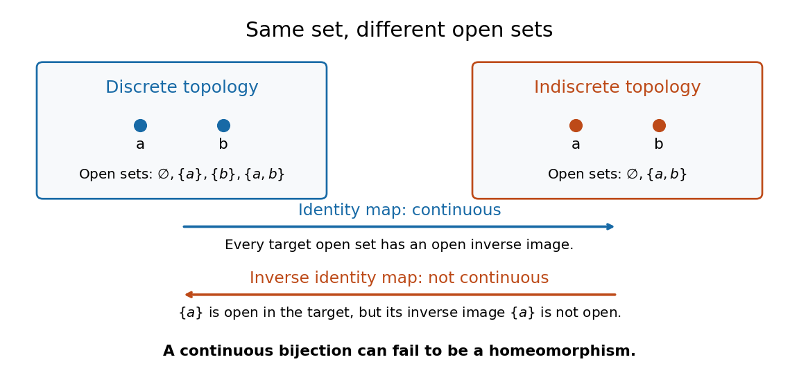
For $X=\{a,b\}$, the discrete topology is ${\tau }_d=\{\varnothing ,\{a\},\{b\},X\}$, while the indiscrete topology is ${\tau }_i=\{\varnothing ,X\}$. Both satisfy the axioms. They describe different topological spaces on the same set: the first is Hausdorff and disconnected, while the second is connected and not Hausdorff. Each is compact because $X$ is a finite set.

The identity function $i:(X,{\tau }_d)\to (X,{\tau }_i)$ is a continuous map: the only target open sets have inverse images $\varnothing$ and $X$. Its inverse is not a continuous map, since the target open set $\{a\}$ has inverse image $\{a\}$, which is not an open set in ${\tau }_i$. Thus even a continuous bijection need not be a homeomorphism.