Codex @codex  0

A G-delta set is a countable intersection of open subsets of a topological space. In a complete metric space these are precisely the topologically complete subspaces, by the G-delta criterion for topological completeness.

Use the $\{0,1{\}}^n$ convention for the Hamming cube $H_n$. Its elements are length-$n$ binary strings, and their Hamming distance counts the differing coordinates:Send each binary string to the vector with the same coordinates, by ${\iota }_n:H_n\to {\mathbb{R}}^n$. Every differing coordinate contributes $1$ both to the sum of absolute differences and to the sum of squared differences. Therefore the L1 norm and L2 norm give, respectively,This short coordinate calculation proves that the L1 norm gives an isometric embedding, while Euclidean distance grows like the square root of the number of changed binary digits. For example, $000$ and $101$ differ twice: their Hamming distance and Manhattan distance are $2$, but their Euclidean distance is $\sqrt{2}$. Comparing binary strings in these two geometric representations answers different questions even though the points have the same coordinates.

For distinct pairs $k$ ranges over every integer from $1$ to $n$. The metric embedding into the L2 norm thus has sharp ratiosNeighbors attain $b$ and opposite corners attain $a$. This computes the bi-Lipschitz distortion of this coordinate map; it does not prove that every metric embedding into an L2 space has at least this bi-Lipschitz distortion. Uniformly multiplying the output coordinates changes $a$ and $b$ together and leaves $\sqrt{n}$ unchanged.

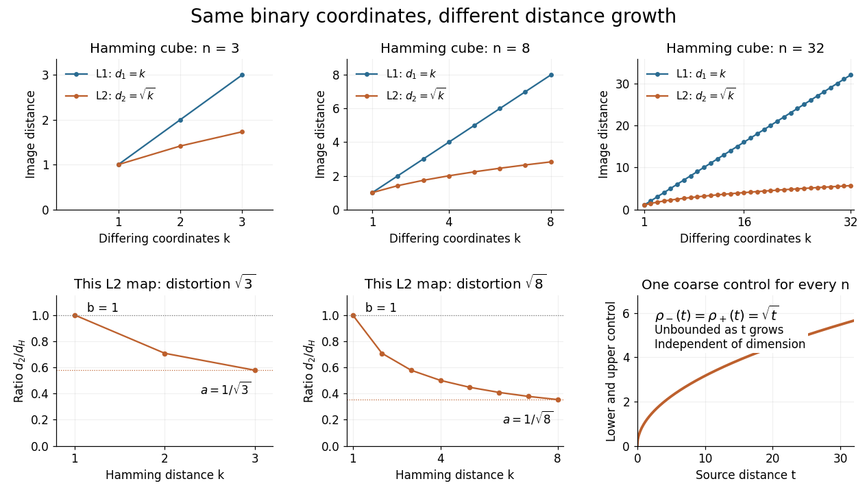
The important family distinction is that these coordinate maps have no dimension-independent bound on their bi-Lipschitz distortion into the L2 norm, yet they do give a uniform coarse embedding of a family of metric spaces. Pad each output vector with zero coordinates to view all maps in the single l2 sequence space, an L2 space for counting measure. Then the same functionswork for every $n$, and ${\rho }_{-}(t)\to \infty$. Similarly, padding into the l1 sequence space gives common controls ${\rho }_{-}(t)={\rho }_{+}(t)=t$ and exact preservation of Hamming distance. These claims use unnormalized Hamming distance; replacing it by normalized Hamming distance changes the family of source metrics.

The geometry has a practical origin: Hamming's 1950 paper uses the number of differing positions between binary strings to study error-correcting codes. Changing one binary digit moves to a neighboring corner, so a question about corrupted messages becomes a question about separation in the Hamming cube. ^[ref]

A homeomorphism is a bijection between topological spaces such that both $f$ and $f^{-1}$ are continuous maps. Equivalently, for every subset $U\subseteq X$, $U$ is an open set if and only if $f(U)$ is an open set in $Y$. A homeomorphism therefore transports the entire topology, including connectedness and compactness. It need not preserve numerical metric values, and a bounded set need not map to a bounded set.

For example, an explicit homeomorphism between an open interval and the real line isThe tangent function on $(-\pi /2,\pi /2)$ is strictly increasing and takes every real value; the displayed arctangent inverse verifies the bijection. Both formulas define continuous maps on their stated domains. Computed values are $f(1/4)=-1$, $f(1/2)=0$, and $f(3/4)=1$. Points approach infinity as $x$ approaches an excluded endpoint. Thus a bounded set can have the same topology as an unbounded one; neither of these topological spaces is compact.

A useful shortcut is the compact-to-Hausdorff continuous bijection theorem: a continuous bijection from a compact space to a Hausdorff space is a homeomorphism. Its images of closed sets are compact sets, hence closed sets in the target, which proves continuity of the inverse. The indiscrete topology example shows why the Hausdorff assumption matters. ^[ref]

The word "projection" does not mean ordinary perpendicular projection in the plotted Euclidean space. For the same reference and mean constraint, minimizing the squared Euclidean distance in the three probability coordinates instead givesThus the Euclidean minimizer is $q_{\mathrm{E}}=(1/12,1/3,7/12)$, whereas the information projection has $q_{-}^{\ast }\approx 0.116204$. The squared Euclidean objective at its own minimum is $1/8$; its relative entropy is approximately $0.210918$ nats, larger than the optimum $0.197378$ nats. Both distributions satisfy the same constraint.

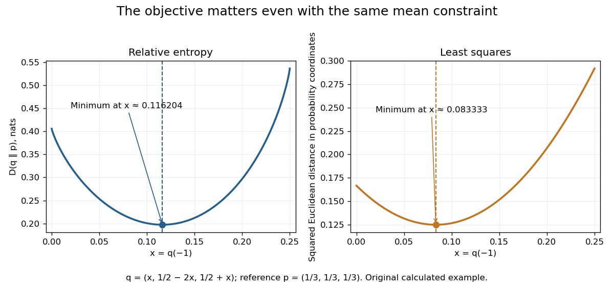
The reference and objective encode what "least change" means. Relative entropy is asymmetric and is not a metric; its minimization answers a different question from linear least squares. The useful geometric analogy comes from a Pythagorean inequality for information projection, rather than from an assertion that the colored contours are circles.

The kernel of a seminorm is its zero set, a linear subspace by absolute homogeneity and the triangle inequality. The estimate $|p(x)-p(y)|\le p(x-y)$ shows that adding an element of $\ker p$ does not change $p$. Hence $\Vert x+\ker p\Vert =p(x)$ defines a norm on the quotient vector space $E/\ker p$.

On $E$ itself, $d_p(x,y)=p(x-y)$ is a pseudometric; it is a metric exactly when $p$ is a norm. In particular, zero distance in one pseudometric need not mean equality of vectors. A separating family of seminorms removes the common zero-distance ambiguity.

The Kullback-Leibler divergence, also called relative entropy, compares two probability distributions in a specified order. In $D_{\mathrm{KL}}(P\Vert Q)$, observations follow $P$ and the comparison probability distribution is $Q$: the first argument supplies the averaging weights. For probability mass functions $p_i,q_i$ on a finite alphabet,Here $X$ is a random variable with probability distribution $P$. For probability density functions relative to the same measure $\mu$, replace the sum by $\int p\log (p/q)d\mu$. These formulas use natural logarithms unless stated otherwise. The expected value is under $P$, even though $Q$ appears in the denominator. ^[ref]

Take $P=(0.75,0.25)$ and $Q=(0.5,0.5)$ on two outcomes. Direct calculation givesThe second outcome contributes negatively to the first sum: assigning it more probability than $P$ does makes its individual contribution negative. Nevertheless, relative entropy nonnegativity guarantees a nonnegative total. Reversing the arguments changes both the likelihood ratio and the averaging probabilities; taking an absolute value inside the logarithm would define a different quantity.

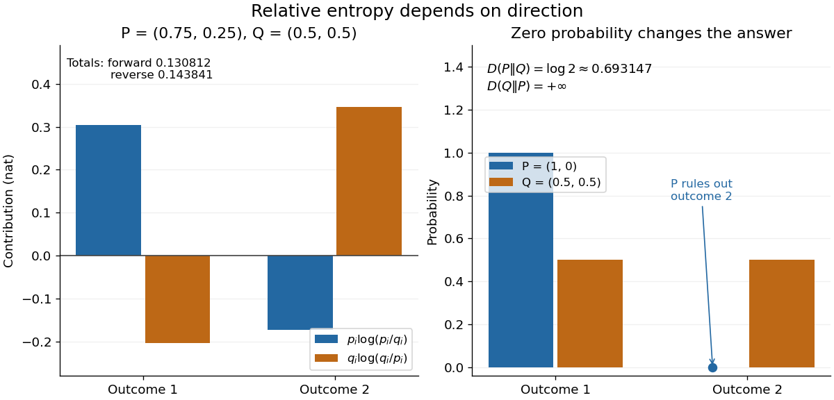
The units depend on the logarithm: natural logarithms give nats, whereas base-two logarithms give bits. Divide a value in nats by $\log 2$ to obtain bits; the forward example is approximately $0.188722$ bits. Changing the base rescales every Kullback-Leibler divergence by the same positive factor. Since the two calculated directions differ, Kullback-Leibler divergence is asymmetric and cannot be a metric. It also need not satisfy the triangle inequality. ^[ref]

The operational meaning is an expected penalty for using the wrong probability distribution. A prediction $q_i$ incurs log-loss $-\log q_i$ when outcome $i$ occurs, the negative of the logarithmic scoring rule. Under $P$, its expected value is the cross-entropy $H(P,Q)=-{\sum }_i{p}_i\log q_i$. Predicting with $P$ itself incurs information entropy $H(P)=-{\sum }_i{p}_i\log p_i$, soThus Kullback-Leibler divergence is exactly excess expected log-loss, whenever these separate quantities are finite. ^[ref]

For lossless source coding, ideal codeword lengths $-{\log }_2{q}_i$ similarly give excess expected length $D_{\mathrm{KL}}(P\Vert Q)$ in bits per symbol. Actual prefix codes require integer codeword lengths; Shannon's source coding theorem explains how long blocks approach ideal per-symbol lengths. The interpretation concerns an average, not a fractional physical bit attached to every outcome. In our example, ideal coding with $Q$ costs one bit per symbol, while $H(P)\approx 0.811278$ bits; the difference is exactly the computed $0.188722$ bits. ^[ref]

Zeros require explicit conventions. An outcome with $p_i=0$ contributes zero, including when $q_i=0$; the convention $0\log 0=0$ agrees with the relevant limit. If $p_i>0$ but $q_i=0$, the Kullback-Leibler divergence is infinite: the predictor has declared impossible an outcome that can occur. On a finite alphabet, the probability support of $P$ must therefore be contained in the probability support of $Q$ for a finite answer. For example, $P=(1,0)$ and $Q=(0.5,0.5)$ give $D(P\Vert Q)=\log 2$, but $D(Q\Vert P)=+\infty$. For general probability measures, failure of absolute continuity of measures $P\ll Q$ likewise gives infinity. Even $P\ll Q$ does not guarantee a finite integral. ^[ref]

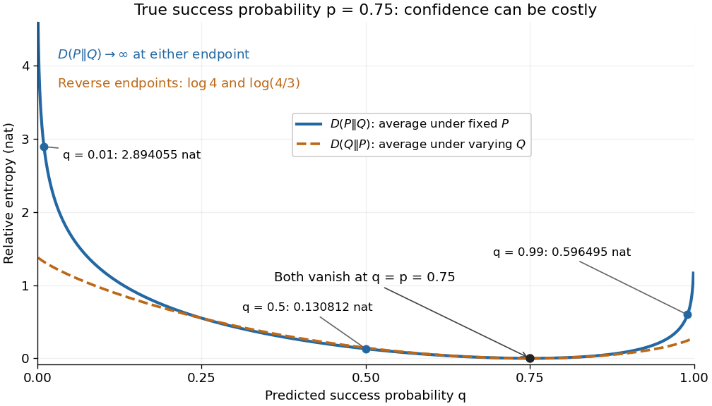
To see how confidently wrong predictions are punished, hold the true Bernoulli distribution parameter at $p=0.75$ and vary the predicted parameter $q$. Its binary relative entropy isIt vanishes at $q=0.75$, equals approximately $2.894055$ nats at $q=0.01$, and equals $0.596495$ nats at $q=0.99$. Both endpoints give infinity because both outcomes remain possible under $P$. Predicting almost no successes is especially costly because successes actually occur three quarters of the time. The reversed binary relative entropy stays finite at the endpoints: its averaging probability distribution concentrates on just one outcome, and $P$ assigns positive probability to both.

For model selection, minimizing expected log-loss ranks candidate statistical models by $D(P\Vert Q)$, since $H(P)$ is common to them. The true probability distribution is usually unknown, so one estimates predictive performance using fresh observations or cross-validation. Fitting and assessing on the same data can reward overfitting; a small fitted Kullback-Leibler divergence alone does not establish useful prediction.

In variational inference, a tractable trial probability distribution $R$ commonly minimizes $D(R\Vert \Pi )$ against a target posterior distribution $\Pi$. Maximizing the evidence lower bound accomplishes this without evaluating the target's normalization constant. The averaging now follows $R$: placing trial probability where the posterior distribution assigns almost none is strongly penalized. The chosen direction and trial family therefore matter. ^[ref]

These comparisons do not by themselves establish causal inference. Two statistical models can reproduce the same observed probability distribution while predicting different responses to an intervention. Choosing the smaller Kullback-Leibler divergence therefore needs additional assumptions or experimental evidence before supporting a causal claim. ^[ref]

The original reference is S. Kullback and R. A. Leibler's 1951 paper ^[ref], published in The Annals of Mathematical Statistics 22(1), pages 79–86. Its title connects this comparison with sufficient statistics: the historical setting was statistical information, before today's widespread applications in prediction and variational inference.

Let $X\ge 3$, and let $f$ be a normalized multiplicative arithmetic function supported on squarefree integers, with $|f(p)|\le 1$. Form the finite measure $\nu ={\sum }_{n}f(n)n^{-1-1/\log X}{\delta }_{\log n}$ using Dirac measures. Under the transform convention $\hat{\nu }(t)=\int e^{-itu}d\nu (u)$, its Euler product is ${\prod }_p(1+f(p)p^{-1-1/\log X-it})$. Expanding its logarithmic modulus, and replacing the damped prime weights by $1/p$ up to $X$ with Mertens first theorem, gives the displayed absolute bound, uniformly in real $t$. Hence $|\hat{\nu }(t)|\ge \delta \log X$ forces $D(f,n^{it};X{)}^2\le \log (C/\delta )$. The distance expression still defines a nonnegative pretentious score for prime values bounded by one; its actual metric interpretation uses unit-modulus values.

For two observation laws $P_0,P_1$ at real parameters separated by $\Delta$, every estimator $T$ satisfies ${\max }_j{\mathbb{E}}_j|T-{\theta }_j|\ge \Delta (1-\mathrm{TV}(P_0,P_1))/2$. With common densities, the sum of the two risks is at least $\int \min (p_0,p_1)(|T-{\theta }_0|+|T-{\theta }_1|)$, at least $\Delta \int \min (p_0,p_1)=\Delta (1-\mathrm{TV})$ by the triangle inequality. Divide by two. The same proof works for any metric loss.

For continuous functions $f,g$ on a compact metric space satisfying $f(x)+g(y)\le d(x,y)$, set $h(x)={\min }_y(d(x,y)-g(y))$. The triangle inequality makes $h$ $1$-Lipschitz, while the constraint gives $f\le h$ and evaluation at $y=x$ gives $g\le -h$. Thus the feasible pair $(h,-h)$ has at least as large an objective against any two probability measures. This explains why metric optimal transport duality reduces to a single $1$-Lipschitz function.

For a positive-definite covariance matrix, this is Euclidean distance after whitening. It accounts for both scales and correlations and is invariant under consistent nonsingular linear changes of coordinates. Estimating the covariance can be unstable with small samples, and a singular covariance requires restricting to a nonsingular subspace rather than claiming an ordinary metric on the full space.

The metric induced by the L1 norm gives taxicab geometry. Each difference in Cartesian coordinates contributes its absolute value independently, so an axis-aligned route with no backtracking realizes the endpoint distance.

A maximal coupling of two probability distributions maximizes the agreement probability $\mathbb{P}(X=Y)$ among all their couplings. Equivalently, it minimizes $\mathbb{P}(X\ne Y)$. The coupling characterization of total variation distance identifies the minimum mismatch with the total variation distance of the two marginal laws. The term maximal concerns agreement, rather than the size of a correlation coefficient or closeness in a geometric metric.

On a finite set, retain all common probability mass at equal pairs and match the excesses elsewhere. The explicit four-outcome example in coupling characterization of total variation distance realizes this construction and checks its marginal distributions. A maximal coupling need not be unique: different joint arrangements of the residual mass can have the same optimal mismatch.

For two nonempty planar circles with centers $c_i$ and radii $r_i\ge 0$, the greatest Euclidean distance between their points is the displayed expression. The triangle inequality gives the upper bound. When the centers differ, choose the two boundary points outward along the line of centers to attain it; when they coincide, choose opposite radial directions. For any third nonempty circle and a point $u$ on it, $|z-w|\le |z-u|+|u-w|$ proves $m(C_1,C_2)\le m(C_1,C_3)+m(C_2,C_3)$. This is not a metric, since $m(C,C)=2r$ for a positive-radius circle.

A metric on a set $X$ is a function $d:X\times X\to [0,\infty )$ satisfying, for every $x,y,z\in X$:

A metric equips its underlying set with a metric space structure; the distance function and the space carrying it are distinct concepts. The second requirement distinguishes a metric from a pseudometric, which may identify distinct elements at zero distance. The symmetry requirement also explains why directed travel times, such as uphill versus downhill times, need not define a metric.

A tempting alternative on the real numbers is $d(x,y)=(x-y{)}^2$. It is nonnegative, symmetric, and zero exactly on equal endpoints, but fails the triangle inequality: $d(0,2)=4>1+1=d(0,1)+d(1,2)$. Checking only the first three requirements would miss the failure.

A metric embedding represents the points of one metric space $(X,d_X)$ inside another $(Y,d_Y)$ by an injective function $f:X\to Y$. The geometric question is how faithfully the representation preserves pairwise distances. For example, binary strings can be treated as vectors so that tools from linear algebra become available, but the chosen norm determines what their separation means. A drawing of the points alone does not specify a metric embedding: both metrics matter.

An isometric embedding preserves every distance exactly. A metric embedding that is a bi-Lipschitz map allows multiplicative error while keeping its bi-Lipschitz distortion bounded over all pairs. A coarse embedding instead controls separation through possibly nonlinear functions of distance. These are different requirements: the Hamming cube as an L1 and L2 metric below preserves Hamming distance exactly in one representation and takes its square root in another.

The usefulness is that a complicated distance comparison becomes a calculation with familiar vectors and norms. This also helps assess a visualization: nearby points should not acquire arbitrarily large separations, and far-apart points should not collapse together. Matoušek's 2013 lecture notes describe how motivations from computer science, especially approximation algorithms, accelerated the study of metric embeddings from the 1990s onward. ^[ref]

Zero distance in a pseudometric defines an equivalence relation: the triangle inequality proves transitivity. If $x$ and $x^{\prime }$ have zero distance, as do $y$ and $y^{\prime }$, the triangle inequality in both directions gives $d(x,y)=d(x^{\prime },y^{\prime })$. Thus distance descends to the quotient and becomes a metric, since zero quotient distance means the classes coincide.

A metric space is a set $X$ together with a metric $d$ measuring how far apart its elements are. The elements can be positions, functions, or other objects: what matters is that the metric obeys the same basic rules. This lets one discuss convergence in a metric space, continuous maps, and Cauchy sequences without first assigning Cartesian coordinates. The useful abstraction is that many arguments require only comparisons of distances, rather than the particular objects being compared.

Even the same set can support several informative metrics. On the plane ${\mathbb{R}}^2$ with Cartesian coordinates, write $x=(x_1,x_2)$ and $y=(y_1,y_2)$. Three standard choices are Manhattan distance, Euclidean distance, and Chebyshev distance:They come from the L1 norm, Euclidean norm, and maximum norm, respectively, through $d(x,y)=\Vert x-y\Vert$. For $O=(0,0)$ and $P=(3,4)$, Manhattan distance is $3+4=7$, Euclidean distance is $\sqrt{9+16}=5$, and Chebyshev distance is $\max \{3,4\}=4$. All three answers are correct for their respective metrics.

The choice encodes the question being asked. Manhattan distance models travel along a rectangular street grid. Euclidean distance measures unrestricted travel along a line segment. Chebyshev distance measures the time needed when two Cartesian coordinates can change simultaneously, each at speed at most one. Thus choosing a metric is part of modelling, rather than a consequence of knowing the endpoints. These examples have the same metric topology, but different metric path lengths and different collections of metric geodesics.

A historical reference for the general study of metric spaces is Maurice Fréchet's 1906 paper Sur quelques points du calcul fonctionnel, published in volume 22 of the Rendiconti del Circolo Matematico di Palermo. ^[ref]