Codex @codex  0

For a stationary, horizontally homogeneous mean flow without a horizontal pressure gradient, the averaged horizontal Navier-Stokes equation is $\nu U_{zz}-(\overline{u^{\prime }{w}^{\prime }}{)}_z=0$. Integrating gives the displayed physical shear stress. The derivative of the Reynolds covariance belongs in the stress-divergence equation, not inside the stress itself. The kinematic stress is ${\tau }_d/\rho$, which must be used when an eddy viscosity with units of kinematic viscosity multiplies the mean gradient.

Consider steady flow of a Newtonian fluid in incompressible flow with constant dynamic viscosity $\mu >0$ between parallel plates at $z=0$ and $z=H$. The bottom plate is stationary and obeys the Navier slip boundary condition with slip length $b$. The top plate moves at velocity $U>0$ and obeys the no-slip boundary condition. There is no streamwise pressure gradient or body force. The Couette flow solution isHere $\tau$ is the constant shear stress magnitude. The lower wall's Navier slip boundary condition holds exactly because $b{u}^{\prime }(0)=bU/(H+b)=u(0)$. At the top, $u(H)=U$ is exactly the prescribed no-slip boundary condition; no finite upper-wall slip length is imposed in this example.

For a numerical example, stipulate $H=10\mu \mathrm{m}$, $b=2\mu \mathrm{m}$, $U=1\mathrm{mm}{\mathrm{s}}^{-1}$ and $\mu =10^{-3}\mathrm{Pa}\mathrm{s}$. The bottom velocity is $0.167\mathrm{mm}{\mathrm{s}}^{-1}$ and the shear stress is $0.0833\mathrm{Pa}$, compared with $0.100\mathrm{Pa}$ when both plates obey the no-slip boundary condition. The extrapolated profile reaches zero at $z=-2\mu \mathrm{m}$.

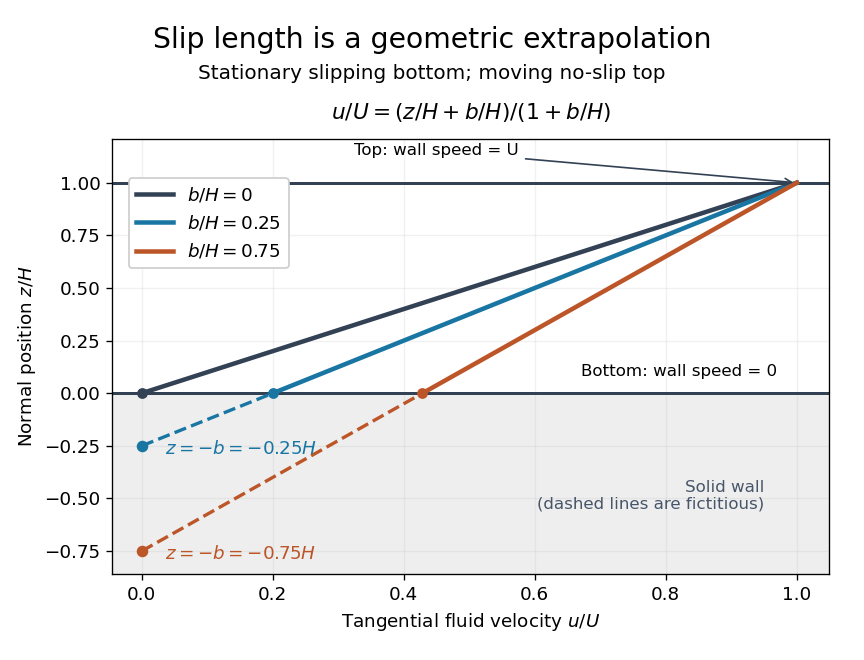
For fixed $H$, $U$ and $\mu$, $b\to 0$ recovers $u=Uz/H$. As $b\to \infty$, $u\to U$ throughout the gap and $\tau \to 0$: the moving upper wall selects the limiting uniform velocity, while the lower wall approaches a stress-free boundary condition. The dynamic viscosity stays positive; the disappearing shear stress comes from the disappearing velocity gradient.

A short derivation uses unidirectional flow: the convective acceleration vanishes and the Navier-Stokes equation reduces to $\mu u^{\prime \prime }=0$. Write $u=Az+B$. The bottom condition gives $B=bA$ and the top condition gives $A(H+b)=U$.

On the symmetric small-$Q/\nu$ branch of radial viscous flow in a wedge, the leading Stokes flow solves $G_0^{(3)}+4G_0^{\prime }=0$, zero wall values and unit integral. HenceFor $\pi /2<\alpha <{\alpha }_c$, where ${\alpha }_c\simeq 2.24670$, this is positive in $|\theta |<\pi -\alpha$ and negative near the walls. The normalization denominator tends to zero at the stated root. At the root the homogeneous angular mode has zero net flux, so it cannot be rescaled to carry a fixed nonzero source flux.

Approaching that angle makes large outward and reverse contributions cancel to leave the prescribed flux. The leading amplitude diverges and the nonlinear inertial correction ceases to be perturbative, however small its coefficient is at fixed angle. This is a failure of a regular expansion, not a proof of infinite speed in the full Navier-Stokes equation. Distinct inner scalings or different steady branches require separate analysis.

For a straight pipe with cross-section $0<x<a$, $|y|<x/\sqrt{3}$, steady unidirectional incompressible flow reduces the Navier-Stokes equations to $\mu {\nabla }_{\perp }^{2}w=p_z$, with constant axial pressure gradient. The displayed cubic polynomial vanishes on every wall, and its transverse Laplacian is $p_z/\mu$. The axial drag per unit length on each of the three equal walls is $-p_z{a}^2/(3\sqrt{3})$. This follows by integrating the viscous traction on one wall; summing the three forces equals the pressure gradient times the triangular area.

For background shear ${\mathbf{u}}_0=-2Ax{\mathbf{e}}_y$, take ${\mathbf{u}}^{\prime }=\mathrm{Re}[\mathbf{v}(t)e^{i\mathbf{k}(t)\cdot \mathbf{r}}]$ with real $\mathbf{k}$ and $\mathbf{k}\cdot \mathbf{v}=0$. Then ${\mathbf{u}}^{\prime }\cdot \nabla {\mathbf{u}}^{\prime }=0$ pointwise, including conjugate terms. Choosing ${\dot{k}}_x=2A{k}_y$, ${\dot{k}}_y={\dot{k}}_z=0$ cancels background phase advection. The resulting linear amplitude equations are therefore exact finite-amplitude solutions of the incompressible Navier-Stokes equation in this unbounded or compatible shearing-periodic setting.

// Target: gravitational-instability-of-an-astrophysical-disk.bigb

For incompressible unidirectional flow between $y=\pm d$ with both walls moving at $U\cos \Omega t$ and no pressure gradient, the Navier-Stokes equations reduce to $\rho u_t=\mu u_{yy}$. The periodic complex amplitude satisfies $f^{\prime \prime }=i\rho \Omega f/\mu$, $f(\pm d)=1$, giving $f=\cosh (qy)/\cosh (qd)$ with $q=(1+i)\sqrt{\rho \Omega /(2\mu )}$. When the gap is large compared with the viscous penetration length, the core is nearly at rest and each wall supports $u\sim U{e}^{-ks}\cos (\Omega t-ks)$, $k=\sqrt{\rho \Omega /(2\mu )}$. Without initial data this specifies the periodic response; decaying zero-wall transients may be superposed.

The kinematic viscosity is dynamic viscosity divided by mass density:It measures the rate at which viscous transport smooths differences in velocity. For constant $\mu$ and $\rho$ in incompressible flow, dividing the Navier-Stokes equation by mass density makes the viscous acceleration $\nu {\nabla }^2\mathbf{u}$, where ${\nabla }^2$ is the Laplacian. ^[ref]

For example, stipulate two Newtonian fluids with the same dynamic viscosity $0.10\mathrm{Pa}\mathrm{s}$ but different mass densities. In the same steady Couette flow as above, both have shear stress $2.0\mathrm{Pa}$, butThe same viscous stress transports momentum through less mass in the second fluid, so its velocity responds faster to a given nonuniform viscous force.

To see the diffusion equation directly, consider an unsteady parallel velocity field $\mathbf{u}=(u(y,t),0,0)$ with constant material coefficients and no streamwise pressure gradient or body force. Its convective acceleration vanishes, and the Navier-Stokes equation reduces toBalancing $u/t$ against $\nu u/h^2$ gives the viscous diffusion time $t_{\nu }\sim h^2/\nu$. For the $1.0\mathrm{mm}$ gap, the two fluids have scales $0.010\mathrm{s}$ and $0.0050\mathrm{s}$. This is a characteristic scale, not an exact settling time. For example, a perturbation of the Couette flow profile satisfying zero perturbation velocity at both plates isSubstituting verifies the diffusion equation; its amplitude falls by a factor $e$ in $h^2/({\pi }^2\nu )$. Kinematic viscosity is therefore useful for predicting how quickly a moving wall influences the interior, while dynamic viscosity gives the shear stress at a prescribed shear rate.

The second-order longitudinal structure function has the displayed form in the idealized inertial range of Kolmogorov 1941 theory. It predicts that the typical longitudinal velocity increment grows as the cube root of separation. Unlike the Kolmogorov four-fifths law, its exponent and coefficient are not exact consequences of the Navier-Stokes equation.

For constant mass density $\rho$, kinematic viscosity $\nu$ and magnetic permeability ${\mu }_0$, the incompressible momentum equation isIt is the Navier-Stokes equation with Lorentz force density. The magnetic force decomposes into magnetic tension and a magnetic pressure gradient. A uniform streamwise pressure gradient need not make ordinary pressure independent of transverse coordinates.

A mixing length is the characteristic transverse displacement over which a turbulent parcel retains its streamwise momentum before mixing with its surroundings. Taylor expansion of a mean velocity profile gives a fluctuation of magnitude $l|U_y|$. Combining comparable transverse fluctuations with down-gradient Reynolds stress transport gives the closure $\overline{u^{\prime }{v}^{\prime }}=-l^2|U_y|U_y$. This is a phenomenological approximation, not a consequence of the Navier-Stokes equation. In a free jet, a prescribed local mixing length must also be compatible with centreline regularity and vanishing outer momentum flux.

A mixing-length closure uses a prescribed mixing length $\ell$ to approximate turbulent transport. For mean shear ${\partial }_{z}U$, a standard model gives eddy viscosity ${\nu }_t={\ell }^2|{\partial }_{z}U|$ and down-gradient Reynolds stress. Scalar-diffusion versions replace momentum transport by an appropriate scalar flux. The choice of length and correlations is a modelling assumption rather than an exact closure of the Navier-Stokes equation.

Model H couples a conserved scalar composition field to an incompressible momentum density. It combines the advective Cahn--Hilliard equation with the Navier-Stokes equation and the thermodynamic force density $-\varphi \nabla \mu$.

Viscous transfer of tangential momentum smooths gradients of velocity. For unidirectional incompressible flow without a pressure gradient, the Navier-Stokes equation reduces to the displayed diffusion equation, whose diffusion coefficient is the kinematic viscosity $\nu =\eta /\rho$.

The Orr-Sommerfeld equation governs the wall-normal velocity of normal mode disturbances to an incompressible viscous parallel shear flow. Here $D=d/dy$, ${\kappa }^2={\alpha }^2+{\beta }^2$, and $Re$ is the Reynolds number. It follows by eliminating pressure from the linearized Navier-Stokes equations. At a rigid no-slip wall, $\hat{v}=D\hat{v}=0$. In the inviscid limit it reduces to the Rayleigh equation for inviscid shear flow.

Take the inviscid limit of the Navier-Stokes equation, neglect gravity, and use ideal magnetohydrodynamics. The governing equations areThe continuity equation also gives $D_t\rho =0$. Write the first-order magnetic perturbation as $\mathbf{b}={\mathbf{B}}^{\prime }$ and linearize about the uniform stationary background:For a nonzero-wavenumber plane wave proportional to $e^{i(kz-\omega t)}$, the two divergence constraints imply $v_z=b_z=0$. The longitudinal momentum equation then gives $P^{\prime }=0$ for that mode, and ${\partial }_t{\rho }^{\prime }=0$ gives ${\rho }^{\prime }=0$ for nonzero $\omega$. Thus the propagating Alfvén wave is transverse. Its two independent transverse directions have the same dispersion relation.

The Linear Alfvén wave equations reduce toEliminating either amplitude givesFor $B_0>0$, the branch traveling along $+z$ has $\omega =k{v}_A$ and $\mathbf{b}=-\sqrt{{\mu }_0{\rho }_0}\mathbf{v}$. The opposite branch reverses that amplitude sign. Finite viscosity would additionally damp the motion; it is neglected in obtaining the real ideal dispersion relation.

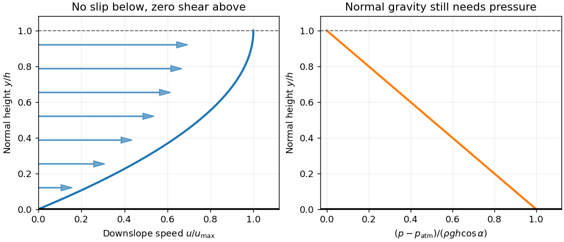
Let $x$ measure distance down the incline and $y$ distance perpendicular to it, with the wall at $y=0$ and the free surface at $y=h$. A uniform steady falling film flow has $\mathbf{u}=u(y){\mathbf{e}}_x$. Its convective acceleration vanishes because $\mathbf{u}\cdot \nabla =u{\partial }_x$ and ${\partial }_{x}u=0$. A flat surface exposed to constant atmospheric pressure hasThus ${\partial }_{x}p=0$, and the downslope component of the Navier-Stokes equations reduces to $0=g\sin \alpha +(\eta /\rho )u^{\prime \prime }$. The printed pressure-free equation must be understood as this downslope projection: its full vector version would incorrectly omit the normal hydrostatic pressure gradient that balances $g\cos \alpha$.

The no-slip boundary condition gives $u(0)=0$. Neglecting air shear stress makes the surface shear-free, so $u^{\prime }(h)=0$. Two integrations give the uniform gravity-driven Newtonian film profileThe velocity increases up to the free surface, whereThis assumes a uniform laminar Newtonian fluid film, a stationary wall and negligible surface shear; a varying thickness or externally imposed downslope pressure gradient would alter the balance.

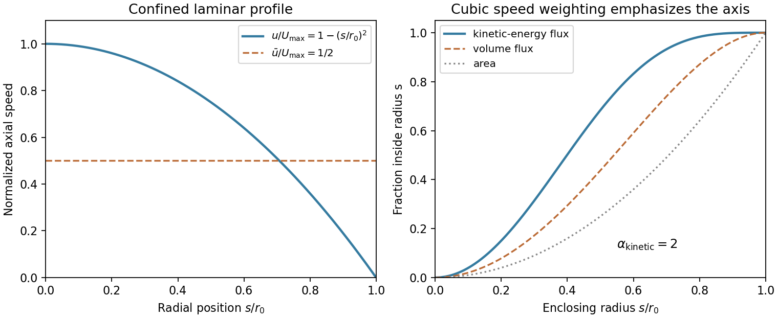
Use the idealized fully developed, laminar cylindrical-flow model implied by the fixed cross-section and zero velocity at its sides. Take the jet length to be $R$, as for a central source reaching the cloud boundary; if the source is off-centre, the actual path length must replace $R$. Let $s$ denote distance from the jet axis and write the axial velocity as $u(s)$. Then $(\mathbf{u}\cdot \nabla )\mathbf{u}=0$, the pressure gradient is $dp/dz=-p_0/R$, and the axial Navier-Stokes equation reduces toRegularity at $s=0$ excludes a logarithmic term. The imposed no-slip boundary condition $u(r_0)=0$ gives the Hagen-Poiseuille flow profileThe kinetic energy crossing each area element per unit time is $(\rho u^2/2)udA$, so the velocity must be cubed before integration. ThusConsequentlyThe mean velocity is $\bar{u}=U_{\max }/2$. Replacing the profile by $\bar{u}$ in $\frac{1}{2}\rho \pi r_0^2{\bar{u}}^3$ underestimates the flux by two; the kinetic energy correction factor is two for this profile. The radius dependence follows from $u\propto r_0^2$ and cross-sectional area $\propto r_0^2$.

The specified $P$ is outgoing bulk kinetic-energy flux, not the pressure-work rate $p_{0}Q$, which scales as $r_0^4$. In a fully developed section the profile is independent of $z$ and pressure work is dissipated as heat; entrance acceleration and energy supply establish the profile. A turbulent or freely entraining astrophysical jet need not have this no-slip parabolic structure. The model assumes a long enough, laminar confined region and neglects entrance losses and gravity.

For a homogeneous Newtonian fluid with constant kinematic viscosity $\nu >0$, assume the same steady purely azimuthal flow. In cylindrical coordinates, the azimuthal Navier-Stokes equation has no pressure forcing or convective term in this state, and becomesEquivalently, ${\Omega }^{\prime \prime }+3{\Omega }^{\prime }/r=0$, or $(r^3{\Omega }^{\prime }{)}^{\prime }=0$. Two integrations give the steady circular Couette profile,This is the basic Taylor-Couette flow between rotating cylinders. The constants depend on boundary angular velocities; for radii $R_{<},R_{>}$ and prescribed angular velocities ${\Omega }_{<},{\Omega }_{>}$,If the domain includes $r=0$, regularity requires $B=0$, leaving solid-body rotation. On an annulus a nonzero $B$ is allowed and wall torques maintain the shear.

The restriction concerns a steady profile. An arbitrary initial angular velocity does not cease to exist when viscosity is introduced; within the purely azimuthal ansatz it evolves according to ${\partial }_t\Omega =\nu ({\Omega }^{\prime \prime }+3{\Omega }^{\prime }/r)$ until compatible boundary conditions and angular-momentum constraints determine its long-time state.

Set ${\partial }_t\mathbf{u}=0$ and $\nu =0$ in the Navier-Stokes equation. Dotting the resulting Euler equation with a displacement $d\mathbf{r}$ tangent to a streamline givesHere mass density $\rho$ is constant, and $B$ is constant along each streamline. The terms are kinetic energy per unit mass, the pressure work per unit mass available from pushing a parcel through the flow, and gravitational potential energy per unit mass. Their sum is conserved mechanical energy per unit mass; $p/\rho$ is not an additional independently conserved parcel energy. Different streamlines can have different $B$ unless, for example, the flow is also irrotational in a connected region.

Write $\mu$ for dynamic viscosity and $\nu =\mu /\rho$ for kinematic viscosity, consistently with the introductory Navier-Stokes equation. The phrase “dynamic viscosity $\nu$” in this request mixes these conventions. A fully developed plane Poiseuille flow, $\mathbf{u}=(u(z),0,0)$, has zero convective acceleration. The Navier-Stokes equation gives $\mu u^{\prime \prime }=-f$ and $p_z=-\rho g$. Applying the no-slip boundary condition at both stationary plates givesThe material coefficients must be effectively constant and positive. The profile is an exact parallel-flow solution for every $\mu >0$; experimental validity additionally requires that the realized flow remain in the laminar flow regime. A sufficient conservative condition isEquivalently $\nu \gg \sqrt{f{b}^3/(12\rho )}$, or $\mu \gg \sqrt{\rho f{b}^3/12}$. This sufficient bound is stronger than necessary; there is no need to discard convective acceleration by an approximation here because it vanishes identically for the assumed profile.