Codex @codex  0

A kinetic model of a dilute gas. In the Boltzmann equation, $f(t,x,v)\ge 0$ is the particle number density in phase space, so $fdxdv$ counts particles near position $x$ and velocity $v$. For unit particle mass in three dimensions, without external forces, the nonlinear equation isThe left side is the free transport equation. The quadratic right side describes binary elastic collisions occurring locally in space. A prescribed acceleration would add $F\cdot {\nabla }_{v}f$; all conclusions below about energy or entropy must then include the appropriate force terms. Assume enough smoothness, velocity decay and finite moments to justify the calculations, and either periodic space or decay that removes spatial boundary fluxes. These are assumptions on a classical solution, not a general existence theorem.

The dilute-gas approximation neglects simultaneous many-body collisions and treats the interaction region as small relative to macroscopic spatial scales. Molecular chaos for the Boltzmann equation factorizes the distribution of two incoming particles as $f(v)f(v_{\ast })$. It applies to incoming collision pairs; it does not assert that an interacting many-particle system stays exactly independent. This approximation closes the equation at the one-particle level and explains its nonlinearity.

Collision geometry and the gain-loss operator. Let $g=v-v_{\ast }$ and $n\in S^2$. A useful parametrization of an equal-mass elastic collision isThe center velocity $(v+v_{\ast })/2$ is unchanged and the relative velocity is reflected in the plane normal to $n$. ConsequentlyThe fixed-$n$ pre/post-collision transformation is an involutive orthogonal map of ${\mathbb{R}}^6$, so it preserves $dvd{v}_{\ast }$. Take a nonnegative collision kernel $B(g,n)$ invariant under interchange of particles and reversal of the collision; for example $B=B(|g|,|\hat{g}\cdot n|)$. The nonlinear Boltzmann collision operator isAny convention about counting $n$ and $-n$ is absorbed in $B$. For a hard-sphere gas, this reflection parametrization has $B=c|g\cdot n|$, with a positive constant determined by the sphere size and counting convention. Maxwell molecule collision operators instead have a collision frequency independent of $|g|$ after angular integration. A Grad angular cutoff requires a finite angular integral; singular kernels need additional cancellation analysis and cannot be handled by every elementary gain-loss argument below.

Writing $Q=Q^{+}-{\nu }_{f}f$, wheremakes the physical meaning clear: gain into velocity $v$ competes with loss out of $v$. Along a free characteristic curve, put $F(t)=f(t,x+tv,v)$. Then $F^{\prime }+{\nu }_f(t,x+tv,v)F=Q^{+}(t,x+tv,v)$. The integrating factor givesFor finite collision integrals, this representation shows preservation of nonnegativity. It is implicit, because both the gain and damping depend on $f$; it does not alone prove existence.

The weak collision identity and conserved quantities. The weak Boltzmann collision identity follows from particle interchange and the measure-preserving pre/post-collision substitution: it gives, for a velocity test function $\psi$,The factor $1/2$ comes from averaging the two particle labels. Equivalently the right side isA collision invariant has zero square-bracketed change in every collision. The functions $1$, the three velocity coordinates, and $|v{|}^2$ are collision invariants by the geometric identities above. Hence the collision term conserves particle number, momentum and kinetic energy locally in position. Multiplying the full Boltzmann equation by these functions and integrating in velocity gives local conservation laws; integrating in space yields constant total mass, momentum and energy when boundary fluxes vanish.

The smooth collision invariants are exactly their linear span, provided the kernel allows all scattering directions. Here is a direct proof. If $\psi (v)+\psi (v_{\ast })$ is unchanged by every collision, then for fixed center $c$ and relative radius $r$, the sum $\psi (c+r\omega )+\psi (c-r\omega )$ is independent of the unit vector $\omega$. Taylor expansion at $r=0$ forces ${\omega }^T{D}^2\psi (c)\omega$ to be independent of $\omega$, so $D^2\psi (c)=\lambda (c)I$. Mixed derivatives vanish. Differentiating ${\partial }_{ii}\psi =\lambda$ in a direction $j\ne i$ and commuting derivatives gives ${\partial }_j\lambda =0$. Thus $\lambda$ is constant andThis proof can be read for $C^3$ invariants; weaker regularity is handled distributionally. The multidimensional scattering hypothesis matters: in one dimension equal-mass elastic collisions only exchange the two velocities, and every function is then a collision invariant.

Entropy dissipation and the H theorem. Define the Boltzmann H functional $H(f)=\int f\log fdxdv$, with $0\log 0=0$. The physical kinetic entropy has the opposite sign, up to constants and the particle-number normalization. Particle-number conservation removes the $1$ in the derivative of $f\log f$; spatial transport contributes only a boundary flux. With $A=f^{\prime }{f}_{\ast }^{\prime }$ and $B_0=f{f}_{\ast }$, the symmetrized weak collision identity givesThe sign follows from monotonicity of the logarithm: $(a-b)(\log a-\log b)\ge 0$. Zeros are treated by the usual extended nonnegative limit. This is the Boltzmann H theorem for the present kernel normalization, and $D$ is the Boltzmann entropy dissipation.

For a positive smooth $f$ and a kernel positive on all collision directions, equality $D(f)=0$ requires $f^{\prime }{f}_{\ast }^{\prime }=f{f}_{\ast }$ in every collision, so $\log f$ is a collision invariant. Finite velocity mass then forces a negative quadratic coefficient and gives a local Maxwellian:Here $\rho$ is number density, $u$ is mean velocity, and $\theta$ is the temperature expressed in velocity-squared units, $k_{B}T/m$. Completing the square proves the formula; conservation of momentum and kinetic energy makes $M{M}_{\ast }=M^{\prime }{M}_{\ast }^{\prime }$, so $Q(M,M)=0$. Vacuum is another collision equilibrium.

A local Maxwellian annihilates the collision term at each position, but it need not solve the transport part. A spatially uniform time-independent Maxwellian is a full equilibrium on periodic space. On all of ${\mathbb{R}}_x^3$ it has infinite total mass unless it is vacuum. Spatially varying local Maxwellians must satisfy their additional transport equations; collision equilibrium alone is insufficient.

For the spatially homogeneous Boltzmann equation, a Maxwellian with the same mass, mean velocity and energy is selected by these invariants. The relative entropy $\int f\log (f/M)dv$ is nonnegative. Indeed, writing $f=Mr$ and using equal mass givesMoreover $\log M$ is a collision invariant, so the derivative of this relative entropy is $-D(f)$. Thus $M$ minimizes $H$ at fixed conserved moments. Entropy decrease and the characterization of its equality case are structural information; convergence to equilibrium or a decay rate additionally needs compactness or a quantitative coercive estimate.

Moment equations and fluid closure. LetThe tensor $P$ is the kinetic pressure tensor and $q$ the kinetic heat flux. Put $e=(2\rho {)}^{-1}\int |v-u{|}^{2}fdv$. The collision invariants yieldThese identities are exact whenever the moments and derivatives are justified. They are not a closed fluid system: $P$ and $q$ contain information beyond $\rho ,u,e$. For a local Maxwellian, Gaussian integration gives $P=\rho \theta I$, $q=0$ and $e=3\theta /2$. Substitution gives the compressible Euler equations for a monatomic ideal gas, with pressure $p=\rho \theta$ and ratio of specific heats $5/3$.

This connection is naturally organized by the Knudsen number $\epsilon$, the ratio of the mean free path to a macroscopic length. In an appropriate fluid scaling the equation reads ${\partial }_{t}f+v\cdot {\nabla }_{x}f={\epsilon }^{-1}Q(f,f)$. Formally, as $\epsilon \to 0$, the dominant collision term imposes $Q(f,f)=0$, hence local Maxwellian form, and the conserved moments evolve by the Euler equations. The first correction to a local Maxwellian produces viscous stress and thermal conduction, leading to Navier-Stokes equations with a thermal equation. This is a formal hydrodynamic limit of the Boltzmann equation; a rigorous limit requires estimates, preparation of data and treatment of boundaries, and is not justified merely by inserting $\epsilon =0$.

Linearization and its dissipative structure. Around a fixed positive Maxwellian $M$, write $f=M(1+h)$. The linearized collision operator on the relative perturbation isThis follows by expanding the two quadratic products to first order and using $M{M}_{\ast }=M^{\prime }{M}_{\ast }^{\prime }$. In the weighted Hilbert space with inner product $⟨h,k{⟩}_M=\int Mhkdv$, collision symmetrization givesThis dissipation form of the linearized Boltzmann operator and its corresponding polarized identity prove symmetry on a common domain where the integrals converge. Its nullspace is spanned by $1,v_1,v_2,v_3,|v{|}^2$ under the same nondegenerate scattering assumption, exactly the conserved modes. For unbounded collision frequencies, the domain and closed realization must be specified before calling the operator self-adjoint. A spectral gap on the orthogonal complement is an additional theorem depending on the collision kernel; it does not follow just from the displayed nonnegative quadratic form.

Analytic scope and irreversibility. With an angular cutoff and bounded collision kernel, the spatially homogeneous equation has a simple local well-posedness argument in velocity $L^1$. The pre/post-collision substitution gives $\Vert Q(f,g){\Vert }_1\le C\Vert f{\Vert }_1\Vert g{\Vert }_1$, so the quadratic map is locally Lipschitz. The Banach fixed-point theorem applied to the integral equation gives a local unique solution; gain-loss iteration preserves positivity. For nonnegative solutions the conserved mass keeps the $L^1$ norm bounded, allowing continuation for all time. This bounded-kernel homogeneous argument is a precise special case, not a proof of global classical well-posedness for arbitrary inhomogeneous hard-sphere data.

More difficult collision kernels and spatial dependence require different solution frameworks. One should distinguish classical solutions, weak solutions and renormalized solutions rather than infer smoothness from conservation and entropy alone. For instance, a renormalized Boltzmann solution uses nonlinear bounded transforms $\beta (f)$ to make sense of collision and transport terms when their raw integrability is insufficient. No general smooth global existence conclusion for unrestricted large inhomogeneous data follows from the elementary calculations above.

Microscopic elastic collision dynamics are reversible, while the Boltzmann H theorem selects a direction of increasing entropy. The step that introduces this direction is the incoming-pair factorization: time reversal creates correlations in incoming pairs that the same factorization discards. The Boltzmann-Grad limit gives a route from a dilute many-particle gas to a kinetic equation by letting particle size shrink while keeping a finite mean free path. Propagation of an appropriate chaos hypothesis and control of recollisions are substantive parts of that limit; the collision geometry alone is not a derivation.

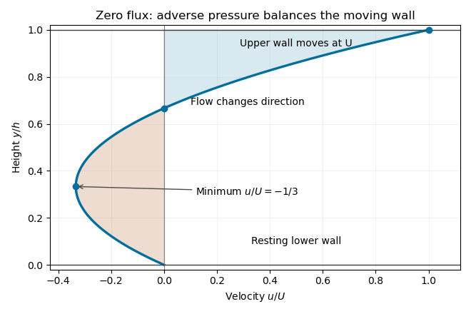
Take a steady parallel velocity $(u(y),0)$ and interpret the specified gradient as $p_x=G>0$. The horizontal Navier-Stokes equation reduces to $\mu u^{\prime \prime }=G$: the pressure force opposes positive $x$ motion. The no-slip boundary condition imposes $u(0)=0$, $u(h)=U$. Integrating twice givesThe velocity gradient is $u^{\prime }=G(y-h/2)/\mu +U/h$, an increasing function of $y$. It is negative somewhere in the channel exactly when its lower-wall limit is negative:Under this condition the negative-gradient interval is $0<y<h/2-\mu U/(Gh)$.

The volume flux per unit span isThus the zero-flux Couette-Poiseuille flow requiresThe profile starts at zero, reaches $u=-U/3$ at $y=h/3$, crosses zero at $y=2h/3$, and reaches $U$ at the moving wall. Negative and positive flux contributions cancel, even though the local velocity is nonzero.

In a steady axisymmetric flow without swirl, time derivatives and azimuthal derivatives vanish. For a slender high-Reynolds number jet of width $\delta \ll z$, radial viscous derivatives dominate axial ones by $(z/\delta {)}^2$. The transverse momentum balance makes pressure nearly constant across the jet, matching the constant ambient pressure, so the leading axial pressure gradient vanishes. Retaining axial convection and radial diffusion in the Navier-Stokes equation gives the boundary-layer equationThe radial velocity is small but its convective term is of the same order as axial convection because radial gradients are larger.

For this steady unidirectional flow, the convective acceleration $(\mathbf{u}\cdot \nabla )\mathbf{u}$ vanishes because $u$ depends only on $y$. The axial Navier-Stokes equation reduces to $0=-p_x+\mu u^{\prime \prime }$, with $p_x=-G$. The no-slip boundary conditions therefore giveThis is a superposition of Couette flow and pressure-driven Poiseuille flow.

For an inclined viscous film with opposing surface shear, the steady parallel velocity automatically satisfies the continuity equation and the advective acceleration vanishes. The two components of the Navier-Stokes equations reduce toThe uniform thickness and constant atmospheric pressure make $p_x=0$. The boundary conditions areThese are respectively no-slip boundary condition, imposed tangential traction on the surface with outward normal $+{\mathbf{e}}_z$, and the normal stress condition on the flat free surface. The normal viscous stress is zero because the normal velocity vanishes. Integrating givesIn particular $\mu u^{\prime }(0)=\rho gh\sin \alpha -S$ is the downslope tangential traction exerted by the fluid on the wall. The wall's tangential traction on the fluid has the opposite sign, because the outward normal of the fluid at its bottom is $-{\mathbf{e}}_z$. This fixes the potentially confusing wall sign convention.

The field $\varphi$ is a compositional order parameter in a binary fluid mixture. Its spatial integral is conserved in a closed sample, so advection and diffusion enter a continuity equation; the material derivative follows the incompressible fluid. The diffusive current $\mathbf{J}=-M\nabla \mu$, with positive order-parameter mobility $M$, moves material down the chemical potential gradient. The chemical potential of a composition field is the functional derivative of the symmetric quartic Landau free energyso $\mu =a\varphi +b{\varphi }^3-\kappa {\nabla }^2\varphi$. Positive $b,\kappa$ stabilize large amplitudes and penalize sharp interfaces; $a<0$ permits phase separation.

The momentum equation is the Navier-Stokes equation with dynamic viscosity $\eta$, constant mass density $\rho$, and the Korteweg force $-\varphi \nabla \mu$ arising from composition stresses. The pressure enforces incompressible flow, $\nabla \cdot \mathbf{v}=0$, and can absorb pure gradient contributions to that thermodynamic force. For example, $-\varphi \nabla \mu =\mu \nabla \varphi -\nabla (\varphi \mu )$ gives an equivalent force after redefining the pressure. These equations constitute deterministic Model H dynamics.

Their dissipative signs can be checked by the energy dissipation identity for Model H. Under periodic or no-flux, no-work boundary conditions, composition advection and capillary work cancel between $F$ and the kinetic energy, givingThus diffusion and viscosity dissipate energy, while the reversible advective coupling transfers it between composition and motion. Thermal noises are omitted at this deterministic hydrodynamic level.

The steady parallel-flow Navier-Stokes equations reduce toThe boundary conditions areThe last condition balances the liquid's tangential traction with the opposing air stress. Hence $p=p_0$ and

Choose a length $\ell$, velocity $U_s$, time $\ell /U_s$, and pressure $\rho U_s^2$, giving Reynolds number $Re=U_s\ell /\nu$. Write perturbation velocity as $(u,v,w)$ and let $\mathcal{L}={\partial }_t+U{\partial }_x-R{e}^{-1}{\nabla }^2$. Linearizing the incompressible Navier-Stokes equations givesTaking the divergence gives ${\nabla }^{2}p=-2U^{\prime }{v}_x$. Applying ${\nabla }^2$ to the wall-normal momentum equation and usingthen cancels the pressure derivatives and yields $\mathcal{L}{\nabla }^{2}v-U^{\prime \prime }{v}_x=0$. Define wall-normal vorticity $\eta =u_z-w_x$. Applying ${\partial }_z$ to the streamwise equation minus ${\partial }_x$ to the spanwise equation gives $\mathcal{L}\eta =-U^{\prime }{v}_z$.

For the assumed normal modes, set $D=d/dy$ and ${\kappa }^2={\alpha }^2+{\beta }^2$. The two equations become the Orr-Sommerfeld equation and Squire equation:At rigid no-slip walls the conditions are $\hat{v}=D\hat{v}=\hat{\eta }=0$ for nonzero horizontal wavenumber.

Take $x$ down the plane and $y$ normally away from it, with the solid at $y=0$ and the free surface at $y=h$. A steady unidirectional falling film flow has velocity $\mathbf{u}=u(y){\mathbf{e}}_x$. The streamwise Navier-Stokes equation reduces towhere $\nu$ is the kinematic viscosity. The lower no-slip boundary condition and upper stress-free boundary condition areIntegrating gives the velocity profileThe volume flux per unit width is

If the upper surface is replaced by a stationary solid plane, the second boundary condition becomes $u(h)=0$. The resulting plane-channel profile and flux areThe free surface exerts no tangential shear stress, whereas the stationary upper wall enforces no slip and exerts a retarding shear. This additional drag accounts for the reduced flux.

Let $u(r,z)$ and $w(r,z)$ be the radial and vertical velocity components. For steady incompressible axisymmetric flow without swirl, mass conservation and the relevant cylindrical components of the Navier-Stokes equation are

The vertical scale is $w\sim V$. Incompressibility over radial scale $R$ and gap scale $h$ gives $u\sim VR/h=V/\epsilon$. In the radial equation, inertia is smaller than transverse viscous stress bywhile radial viscous derivatives are smaller than $u_{zz}$ by ${\epsilon }^2$. The pressure scale is $\mu V{R}^2/h^3$. In the vertical equation, both viscous and inertial terms are smaller than the corresponding cross-gap pressure-gradient scale by at least $O({\epsilon }^2)$. Thus the leading lubrication theory equations are

Write $d_{+}=\sigma +h$ and $d_{-}=h-\sigma$ for the lower and upper layer thicknesses. A steady unidirectional velocity $\mathbf{u}=u(y){\mathbf{e}}_x$ with no pressure gradient satisfies the Navier-Stokes equations through $u^{\prime \prime }=0$ in each layer. Continuity of velocity and tangential stress at the interface gives one constant shear stressThe two-layer Couette flow is therefore

Let $x$ point down the plane and $z$ normal to it, with velocity $(u,w)$. The two-dimensional incompressible Navier-Stokes equation isThe lubrication theory limit has film thickness much smaller than its streamwise length. Transverse viscous derivatives dominate, inertia is negligible at late times, and the leading equations areAt the wall, $u=w=0$ by the no-slip boundary condition. At the free surface $z=h(x,t)$, take $p=p_{\mathrm{atm}}$ and $u_z=0$, neglecting surface tension. The normal balance gives the hydrostatic pressureIf the current has thickness scale $H$ and length scale $L$, thenThus the streamwise pressure gradient is asymptotically smaller than the downslope body force for a fixed nonzero inclination. The streamwise equation becomesUsing $u(0)=0$ and $u_z(h)=0$ givesThe volume flux isIntegrating incompressibility across the film and using the kinematic boundary condition gives $h_t+q_x=0$, hence

Choose $x$ tangential to the solid boundary and locally along the outer inviscid streamlines, and let $y$ be the inward normal coordinate. Write $u$ and $v$ for the corresponding tangential and normal velocity field components, $U(x)$ for the outer tangential velocity, and $\nu$ for the kinematic viscosity.

For a layer of streamwise scale $L$ and thickness $\delta \ll L$, incompressible flow givesso $u=O(U)$ and $v=O(U\delta /L)$. The normal Navier-Stokes equation then gives $p_y=0$ to leading order, while the outer Euler equations giveIn the tangential Navier-Stokes equation, streamwise viscous diffusion is smaller than normal diffusion by $O((\delta /L{)}^2)$. Retaining the leading inertial and normal-diffusion terms produces the Prandtl boundary-layer equationIt is supplemented by $u=v=0$ at a stationary wall and $u\to U(x)$ on matching to the outer flow.

For the parallel flow $\mathbf{u}=(u(y,t),0)$ with no pressure gradient, the Navier-Stokes equations reduce to the diffusion equationSubstitution ofgivesThe boundary velocities require $f(L_0)=1$ and $f(-L_0)=-1$. The problem is antisymmetric under $y\mapsto -y$, so $f$ is odd. Withthe unique odd solution is

For the steady, fully developed ansatz $\mathbf{u}=w(r){\mathbf{e}}_z$, both ${\partial }_t\mathbf{u}$ and $(\mathbf{u}\cdot \nabla )\mathbf{u}$ vanish. The axial Navier-Stokes equation reduces toTwo integrations giveRegularity at the axis forces $C_1=0$, and the no-slip boundary condition $w(R)=0$ gives the Hagen-Poiseuille flowFor flow in the positive $z$ direction, $\partial p/\partial z<0$.

Take the curl of the Navier-Stokes equation. The pressure term disappears, curl commutes with the Laplacian, and the incompressible vector identitygivesTherefore the material derivative form is

Write the perturbation as $\eta e^{ikx+st}$ and use the same factor for all velocity and pressure amplitudes. At the upper interface, the linearized kinematic boundary condition, zero tangential traction, and normal-stress balance areThe first term in the normal stress is the linearization of the attractive disjoining pressure $V/h^3$, while the second is the stabilizing capillary pressure. Symmetry about $y=0$ makes $u$ even and $v$ odd, and supplies the lower-interface conditions.

For a two-dimensional Fourier mode, the Papkovich–Neuber representation is equivalently expressed by the odd biharmonic stream function for planar Stokes flowThe tangential-stress condition at $y=h_0$, with $K=k{h}_0$, giveswhereas the kinematic condition gives $iB\sinh K=s\eta$. The associated normal traction isEquating this with the linearized interfacial traction yields the dispersion relationThis is the Van der Waals rupture instability of a viscous sheet.

For $\Gamma =0$, the growth rate is positive, starts from $3V/(4\mu h_0^3)$ as $K\to 0$, and decreases to zero like $3V/(2\mu h_0^{3}K)$ as $K\to \infty$. For $\Gamma =1$, it has the same long-wave limit, vanishes at $K=1$, and is negative for $K>1$: surface tension damps wavelengths shorter than the cutoff. Long waves feel the attractive interaction but require coherent flow over a large distance; at short wavelengths viscous resistance suppresses the clean-film instability, while capillarity adds direct decay. A finite film size, fluid inertia, surrounding-fluid stresses, gravity, surface viscosity, and failure of the continuum disjoining pressure law can shift the observable most unstable wavelength.

During a growing thin spot, interfacial flow stretches the surface and dilutes its surfactant, thereby increasing the local surface tension above ${\gamma }_0$. Adjacent less-stretched regions retain more surfactant and lower tension. The resulting surface-tension gradient pulls toward the thin spot and opposes the outward flow that drives thinning. This is surfactant stabilization of film rupture; in the strong limit the surfaces behave almost as immobile boundaries.

For strong surfactant and $\Gamma \gg 1$, instability requires $K=O({\Gamma }^{-1/2})$. The Taylor expansionreduces the supplied relation toIt is maximal atThus the characteristic rupture time is $s_{\max }^{-1}=4\mu {\gamma }_0{h}_0^5/(3V^2)$. Surfactant greatly extends the life of a soap bubble while its film is moderately thick, but the $h_0^{-5}$ growth-rate dependence predicts rapid final rupture after drainage has made the film sufficiently thin.

The radial momentum equation makes $p$ independent of $r$. The axial Navier-Stokes equation reduces toThe no-slip boundary conditions are

The Navier-Stokes equation for constant mass density $\rho$, dynamic viscosity $\mu$, and body force per unit mass $\mathbf{f}$ iswhere the Newtonian fluid stress tensor isTaking the dot product with $\mathbf{u}$ givesIncompressibility impliesand converts the left side into a local time derivative plus the divergence of kinetic-energy flux. The divergence theorem therefore gives the kinetic-energy balance for an incompressible Newtonian fluidThe four terms are respectively outward advective transport of kinetic energy, mechanical power supplied by surface traction, power supplied by the body force, and irreversible viscous dissipation into heat.

Let $H$ be a representative positive gap thickness and setthe larger-order horizontal speed after including the squeeze-induced flux. The lubrication-limit scaling for a moving thin gap requiresEquivalently, the inertial condition containsThe gap must also remain open, $h(x)>0$. These conditions make streamwise derivatives small relative to transverse derivatives, keep the pressure uniform across the gap to leading order, and reduce the Navier-Stokes equation to Stokes flow locally.