Codex @codex  0

A stationary iterative method for a linear system converges to its specified fixed point for every initial vector if and only if its iteration matrix satisfies $\rho (H)<1$, where the spectral radius is the largest modulus of an eigenvalue.^[ref]

For a diagonalizable matrix, write $H=V\Lambda V^{-1}$. Then $H^k=V{\Lambda }^k{V}^{-1}$, so each eigenvector coefficient tends to zero exactly when its eigenvalue has modulus less than one. For a general matrix, the Jordan normal form gives the same result: a Jordan block $J=\lambda I+K$ with a nilpotent matrix $K$ of size $m$ satisfiesIf $0<|\lambda |<1$, every coefficient tends to zero because exponential decay beats any fixed polynomial in $k$; if $\lambda =0$, the block vanishes once $k\ge m$. Conversely, an eigenvector with $|\lambda |\ge 1$ provides an initial error that cannot tend to zero. For a real matrix with complex eigenvalues, the same obstruction appears in the real invariant subspace spanned by the real and imaginary parts of an eigenvector.

The words "every initial vector" matter. For example, $H=\mathrm{diag}(3/2,1/2)$ fails the criterion, but $e^{(0)}=(0,1{)}^T$ still tends to zero. Here a generic initial error has a nonzero first coordinate and diverges; the exceptional errors lie on the second coordinate axis. With $H=\mathrm{diag}(-1,1/2)$, generic errors oscillate rather than diverge in norm, while the same exceptional axis still converges. Both are valid matrix splittings with $M=I$ and $A=I-H$. In general the convergent errors form the direct sum of the generalized eigenspaces for $|\lambda |<1$; if $\rho (H)\ge 1$, this is a proper linear subspace.

A small spectral radius describes eventual convergence, but does not imply that the Euclidean norm of the error decreases on every step for a non-normal matrix. An operator norm bound $\Vert H\Vert <1$ does give the stepwise estimate $\Vert e^{(k)}\Vert \le \Vert H{\Vert }^k\Vert e^{(0)}\Vert$. For a real symmetric matrix, the matrix 2-norm equals its spectral radius, making this particularly direct.

If $\mathrm{Re}⟨Lv,v⟩\le 0$ in a finite-dimensional Hilbert space, $I-hL/2$ is invertible for every positive $h$. The relation $v_{+}-v_{-}=(h/2)L(v_{+}+v_{-})$ gives $\Vert v_{+}{\Vert }^2-\Vert v_{-}{\Vert }^2=(h/2)\mathrm{Re}⟨L(v_{+}+v_{-}),v_{+}+v_{-}⟩\le 0$. Thus the Crank-Nicolson method contracts for such a linear system even when $L$ is a non-normal matrix. This is a direct energy result, not an unqualified inequality by a scalar rational function evaluated at a logarithmic norm.

A nonlinear term $f(|x|)Nx$ with real skew-symmetric matrix $N$ contributes zero to the derivative of the quadratic energy $|x{|}^2/2$. It changes orientation rather than magnitude directly. If a separate linear generator is a non-normal matrix, that reorientation can still alter later transient growth, so energy cancellation alone does not make the nonlinear evolution equivalent to the linear one.

The spectral radius of the matrix exponential gives the lower bound through the spectral abscissa $s(A)$. Differentiating the squared Euclidean norm along $q^{\prime }=Aq$ and bounding its Hermitian quadratic form gives the upper bound through the Euclidean logarithmic norm ${\mu }_2(A)$. A non-normal matrix can have ${\mu }_2(A)>0$ despite $s(A)<0$, allowing transient growth before its ultimate decay.

The Floquet growth rate measures the exponential trend of a periodic linear differential equation over many coefficient periods. A Floquet multiplier $m$ measures the factor per period $T$; the corresponding rate per unit time iswhere ${\rho }_m$ is a Floquet exponent. Taking the real part removes the ambiguity in the complex logarithm.

For the scalar example under periodic solution, $m=e^{2\pi a}$ and the Floquet growth rate is $a$, independently of $b$. Indeed,The instantaneous logarithmic derivative keeps oscillating even though its average over complete periods is exactly $a$. Sampling at the same phase in each period removes the modulation altogether: $y(nT)=m^{n}y(0)$.

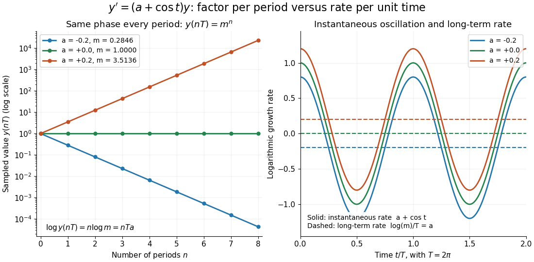
For the general finite-dimensional homogeneous linear differential equation $x^{\prime }=A(t)x$, assume that $A$ is continuous on the real line and $T$-periodic, with $T>0$. Normalize its fundamental matrix by $\Phi (0)=I$ and set $M=\Phi (T)$. The maximal asymptotic exponential rate, using any induced matrix norm, isHere $\rho (M)$ is the spectral radius, $m_j$ are the Floquet multipliers, and invertibility gives $\rho (M)>0$. This concerns growth of the solution operator; it does not say that every initial condition attains the maximum.^[ref]

To prove the formula, write $t=nT+s$ with $0\le s<T$. Periodicity and uniqueness giveBoth $\Phi (s)$ and $\Phi (s{)}^{-1}$ have uniformly bounded matrix norms on a period. Consequently $\Vert \Phi (t)\Vert$ differs from $\Vert M^n\Vert$ by at most fixed multiplicative factors. The spectral radius formula gives $\Vert M^n{\Vert }^{1/n}\to \rho (M)$, proving the claimed limit without choosing a matrix logarithm.

For a particular nonzero initial condition $v$, decompose $v$ into the generalized eigenspaces of $M$ over the complex numbers. The rate of $\Phi (t)v$ is the largest $T^{-1}\log |m_j|$ among components that are nonzero. Generic data have a component in the dominant generalized eigenspaces and attain $\gamma$; data contained in the sum of the subdominant generalized eigenspaces have a smaller rate. For example, with $A=\mathrm{diag}(0.2,-0.3)$, the maximal rate is $0.2$, while $v=(0,1)$ decays at rate $-0.3$. These invariant subspaces describe initial data at phase zero. Their transported versions $E(t)=\Phi (t)E(0)$ can vary with time and satisfy $E(t+T)=E(t)$.

A negative Floquet growth rate allows temporary amplification. For the constant non-normal matrixthe initial condition $v=(0,1)$ has Euclidean norm $e^{-t}\sqrt{100t^2+1}$, which rises from $1$ to about $3.697$ at $t=1$ before eventually decaying. Its exponential rate is still $-1$: the Jordan block contributes a polynomial factor, whose logarithm divided by $t$ tends to zero. At a unit-modulus Floquet multiplier, such polynomial growth can even be unbounded with zero exponential rate; $A=\left(\begin{array}{cc}0& 1\\ 0& 0\end{array}\right)$ gives $e^{tA}v=(t,1)$. Thus zero Floquet growth rate alone proves neither boundedness nor a periodic solution.

For $x^{\prime }=Lx$ and $E=\Vert x{\Vert }_2^2$, the Hermitian matrix $H=(L+L^{\ast })/2$ gives $\dot{E}=2x^{\ast }Hx$. Thus some initial condition grows immediately iff the largest eigenvalue of $H$ is positive. All trajectories have nonincreasing energy iff $H$ is a negative semidefinite matrix. This differs from requiring negative real parts for the eigenvalues of $L$: a non-normal matrix can satisfy modal decay while allowing transient growth.

For $L=\left(\begin{array}{cc}-1/R& 1\\ 0& -1/(4R)\end{array}\right)$ with $R>1$, put $s=\sqrt{1-R^{-2}}$ and $q=(5-3s)/(5+3s)$. The optimal energy amplification of a linear system reaches its maximum atThe maximizing initial orientation is ${\rho }^{+}$ and the final orientation is ${\rho }^{-}$ from the orientation interval for transient energy growth. Taking $R\to \infty$ gives the displayed viscous-time and Reynolds-squared asymptotics. These constants belong to this specified triangular model, not to every non-normal matrix.

Take the norm to be the Euclidean norm. The solution is $\mathbf{q}(t)=e^{tA}\mathbf{q}(0)$, so optimal growth is the operator norm $G(t)=\Vert e^{tA}{\Vert }_2$, equivalently the largest singular value of the matrix exponential. Let $s(A)$ be the spectral abscissa and let $w(A)={\lambda }_{\max }((A+A^{\ast })/2)$ be the numerical abscissa. The Euclidean semigroup growth bounds areFor the lower bound, the spectral radius of $e^{tA}$ is $e^{ts(A)}$ and is bounded by its operator norm. For the upper bound, differentiating $\Vert \mathbf{q}{\Vert }_2^2$ gives $2\mathrm{Re}({\mathbf{q}}^{\ast }A\mathbf{q})\le 2w(A)\Vert \mathbf{q}{\Vert }_2^2$, and integration gives the result. A non-normal matrix can have $w(A)>s(A)$, allowing transient amplification even when all its eigenvalues have negative real parts.

For the triangular matrix, $s(M)=-1/R$. The eigenvalues of its Hermitian part are $-3/(2R)\pm \frac{1}{2}\sqrt{1+R^{-2}}$, soThe upper exponent becomes positive when $R>\sqrt{8}$, even though the long-time spectrum is stable.

The two equations are $q_1^{\prime }=-q_1/R$ and $q_2^{\prime }=q_1-2q_2/R$. Solve the first, then use an integrating factor in the second. Writing $s=t/R$, $a=e^{-s}$, $b=e^{-2s}$ and $c=R(a-b)$ givesThe maximizing initial state is the unit eigenvector of $B^{\ast }B$ belonging to its largest eigenvalue. HereFor $t>0$, defineThe optimal initial state for triangular stable shear is thereforeMultiplication by any nonzero complex scalar gives the same growth ratio; at $t=0$, every nonzero initial state is optimal.

For $t\gg R$, $d\to \infty$ and $r\to 0$. Thus the optimal initial state tends to $(1,0{)}^T$, and $G(t)\sim e^{-t/R}\sqrt{1+R^2}$. The initial first component excites the slower eigenmode and its amplified second component.

For $t\ll R$, the exact expression gives $d=(R^{-1}+t/2)[1+O(t/R)]$. Accordingly the short-relative-time optimal state for triangular shear usesThis retains both the unequal damping rates and the shear. If $R\gg 1$, it reduces to $r\sim (\sqrt{t^2+4}-t)/2$, the maximizing direction for the shear matrix $\left(\begin{array}{cc}1& 0\\ t& 1\end{array}\right)$. If time also tends to zero at fixed $R$, it instead tends to $r=\sqrt{1+R^{-2}}-R^{-1}$, the largest-eigenvalue direction of the Hermitian part of $M$. Merely setting $t/R$ small does not justify setting $t$ small; the exact formula resolves both possibilities.

A stiff differential equation can contain rapidly decaying modes as well as a slowly changing solution of interest. An explicit scheme may need a very small step solely to keep those already small fast modes from numerical growth. A-stability addresses this restriction through the Dahlquist test equation $y^{\prime }=\lambda y$, whose exact solution decays when $\mathrm{Re}\lambda <0$.

For a one-step method, write $y_{n+1}=R(z)y_n$, $z=h\lambda$. Its linear stability domain consists of the points where the update is defined and $|R(z)|\le 1$. A-stability means that this domain contains the closed left half-plane. This is a scalar linear stability property, not an order condition, an existence theorem for an implicit solve, or a general nonlinear contractivity assertion.

For a rational approximation to the exponential, consistency requires $R(z)=1+z+O(z^2)$, and order $p$ requires $R(z)-e^z=O(z^{p+1})$. Poles must be absent from the relevant half-plane. The Forward Euler method has $R=1+z$ and the disk $|1+z|\le 1$, so negative real modes require $h|\lambda |\le 2$; it is not A-stable. The Backward Euler method has $R=(1-z{)}^{-1}$, and $|1-z|\ge 1$ on the left half-plane, so it is A-stable. The trapezoidal rule and the implicit midpoint rule both have, on the scalar linear problem,They are second-order and A-stable despite being different nonlinear methods. No nonconstant polynomial approximation is A-stable, because its modulus grows without bound on the negative real axis. In particular every nontrivial explicit Runge-Kutta method has a bounded-step stability restriction.

A-stability prevents growth but need not eliminate extremely stiff modes: the trapezoidal factor tends to minus one as $z\to -\infty$. L-stability additionally requires $R(z)\to 0$ within the left half-plane. Backward Euler is L-stable; trapezoidal and implicit midpoint are not. The distinction explains persistent alternating transients in otherwise stable Crank-Nicolson calculations. Accuracy still constrains useful step sizes even for an A-stable method.

A linear multistep method is characterized by polynomials $\rho ,\sigma$, and its scalar modes satisfy $\rho (\zeta )-z\sigma (\zeta )=0$. There is generally no single scalar amplification factor: every root must lie in the closed unit disk and unit roots must be simple. At $z=0$, this is the zero-stability root condition. Consistency plus zero-stability gives convergence by the Dahlquist equivalence theorem, with suitable starting values. A-stability demands the amplification root condition throughout the left half-plane, including the zero-step condition. The Second Dahlquist barrier says that an irreducible A-stable linear multistep method has order at most two, and an explicit linear multistep method cannot be A-stable.

Examples include backward Euler, trapezoidal, and the second-order backward differentiation formulaIts zero-step roots are $1,1/3$. Its unit-circle boundary quotient has real part $(1-\cos \theta {)}^2\ge 0$, and the leading coefficient is nonzero on the left half-plane, giving A-stability by the same continuation argument as in Question 2. Conversely the third-order member of that question fails A-stability. A formal high order without zero-stability, or after silently cancelling a problematic unit factor, does not evade the barrier.

For an implicit Runge-Kutta method, the stages on the test equation satisfy $Y=e{y}_n+zAY$. Whenever these stages are solvable, its stability function isThis rational function is used to test scalar A-stability; the Butcher order conditions separately establish nonlinear order. The Lobatto IIIA method in Question 3 is an A-stable fourth-order example with $R$ the diagonal degree-two Padé approximant. More generally the $s$-stage Gauss--Legendre Runge-Kutta method has order $2s$ and is A-stable, with the diagonal Padé approximation to $e^z$; its stiff-limit factor is nonzero. The $s$-stage Radau IIA method has order $2s-1$ and is L-stable. Thus Runge-Kutta stages permit arbitrarily high A-stable order, unlike irreducible linear multistep formulas.

For a normal matrix, scalar amplification bounds transfer through unitary diagonalization. For a non-normal matrix, eigenvalue information alone does not assert Euclidean contraction: transient growth and eigenvector conditioning can matter. Direct energy method arguments, such as the dissipative Cayley-transform proof in Question 1, use the symmetric part and are more informative in that setting.

For nonlinear dissipative vector fields, the stronger B-stability property asks that distances between two numerical solutions not increase. A standard sufficient condition for Runge-Kutta methods is algebraic stability: $b_i\ge 0$ andis positive semidefinite. It follows from the Runge-Kutta contractivity identity when the implicit stages exist. The three-stage Lobatto IIIA method is A-stable but has the first diagonal entry of that matrix equal to $-1/36$, so scalar A-stability should not be confused with that sufficient nonlinear condition. Stage solvability of an implicit Runge-Kutta method remains a separate issue and computational cost of the implicit equations must be considered. A-stability removes a scalar decay-mode stability restriction; order, stiff damping, nonlinear stability and solvability remain distinct properties.

Both eigenvalues of the linear generator, $-1/R$ and $-1/(4R)$, are negative. Nevertheless the non-normal matrix transfers the slowly decaying second component into the first before viscous decay wins. Modal decay coexists with energy amplification of order $R^2$ over a time of order $R$.

This illustrates transient growth from non-normal modes: large Reynolds number permits much greater disturbance amplification even though the linear stability analysis finds no unstable eigenvalue. The energy-neutral rotational nonlinearity can redirect the amplified state and affect its subsequent evolution. The linear gain alone establishes neither sustained nonlinear instability nor a nonlinear transition threshold.

For $q(t)=B{q}_0$, the energy ratio is the Rayleigh quotient of the Hermitian positive-definite matrix $B^{†}B$:Expanding $q_0$ in the orthonormal right singular vectors makes this a weighted average of ${\sigma }_j^2$. HenceAny nonzero vector in the largest right-singular subspace is optimal if ${\sigma }_1$ is repeated. Its amplified state is proportional to the paired left singular vector. For a non-normal matrix $L$, this optimal initial direction need not be an eigenvector of $L$, explaining transient growth from non-normal modes.

An $s$-stage Runge-Kutta method for $y^{\prime }=f(t,y)$ is defined byThe Butcher tableau records $A=(a_{ij})$, $b$ and $c$; internal consistency usually sets $c=Ae$, and first-order consistency requires $b^{T}e=1$. A strictly lower triangular $A$ gives an explicit method, while other stage dependencies generally require an implicit Runge-Kutta method. The stage solvability of an implicit Runge-Kutta method must be checked separately: if $f$ is globally Lipschitz continuous in $y$ with constant $L$, the stage fixed-point map is a contraction in the maximum stage norm whenever $hL{\max }_i{\sum }_j|a_{ij}|<1$. This is a sufficient small-step condition, not a restriction intrinsic to the definitions of A-stability or B-stability.

Linear stability begins with the Dahlquist test equation $y^{\prime }=\lambda y$. Solving the stages givesThe linear stability domain consists of test values for which the stage system is well defined and $|R(z)|\le 1$. A-stability means this includes the closed left half-plane. For $\mathrm{Re}\lambda <0$, this gives stability with no scalar decay-mode step restriction. For a normal matrix $L$ in $y^{\prime }=Ly$, unitary diagonalization of a normal matrix reduces the norm estimate to these scalar factors. For a non-normal matrix, eigenvalues alone do not establish a uniform norm bound: eigenvector conditioning and transient amplification matter. Mesh-uniform estimates for discretized PDEs must control operator powers, not only their spectra.

Every consistent explicit Runge-Kutta method has a nonconstant polynomial stability function and therefore cannot be A-stable, since that polynomial is unbounded on the negative real axis. For example, Forward Euler method has $R(z)=1+z$, stability disk $|1+z|\le 1$, and restriction $0\le hq\le 2$ for $\lambda =-q<0$. For a pure imaginary mode $\lambda =i\omega \ne 0$, $|1+ih\omega |>1$, so it is unstable for every positive step. The classical fourth-order Runge-Kutta method instead hasIt is stable on the imaginary axis exactly for $|q|\le 2\sqrt{2}$, an illustrative conditional stability range for oscillatory evolution.

Backward Euler method has $R(z)=(1-z{)}^{-1}$ and is A-stable. L-stability adds $R(z)\to 0$ as $|z|\to \infty$ in the left half-plane; backward Euler satisfies this and strongly damps unresolved rapidly decaying modes in a stiff differential equation. The implicit midpoint rule and the trapezoidal rule both have $R(z)=(1+z/2)/(1-z/2)$, so they are A-stable but not L-stable. They preserve the modulus of a pure imaginary test mode, but their stiff-decay limit is $-1$, leaving oscillatory numerical remnants. The three-stage Lobatto IIIA method has the fourth-order rational function found in Question 2 and likewise lacks L-stability. Thus high order and A-stability do not themselves imply efficient stiff damping.

Nonlinear stability measures differences between solutions of the same equation. A one-sided Lipschitz condition isDifferentiating the squared difference and applying the Gronwall inequality gives $\Vert y(t)-\tilde{y}(t)\Vert \le e^{\nu (t-t_0)}\Vert y(t_0)-\tilde{y}(t_0)\Vert$. A dissipative vector field has $\nu \le 0$ and is contractive. A B-stable method preserves this property for every positive step size for which the stages are well defined:This includes time-dependent vector fields when dissipativity holds at each common time argument. Applying it to scalar linear dissipative fields shows that B-stability implies A-stability when the linear stages are well defined; the converse fails.

The standard sufficient theorem is algebraic stability implies B-stability, subject to stage solvability. Define $B=\mathrm{diag}(b)$ and $M=BA+A^{T}B-b{b}^T$. Algebraic stability of a Runge-Kutta method means $b_i\ge 0$ and $M$ is a positive semidefinite matrix. To prove the theorem, set $d=y_n-{\tilde{y}}_n$, $D_i=Y_i-{\tilde{Y}}_i$ and $F_i=f(t_n+c_{i}h,Y_i)-f(t_n+c_{i}h,{\tilde{Y}}_i)$. Expanding the output difference and using $D_i=d+h{\sum }_j{a}_{ij}{F}_j$ yields the Runge-Kutta contractivity identityDissipativity makes the first sum nonpositive, while positive semidefiniteness makes the last quadratic form nonnegative. The latter follows by factoring $M=Q^{T}Q$ and writing it as a sum of squared norms of linear combinations of the $F_i$. This proves the claimed contraction. It is a sufficient theorem; absence of algebraic stability is not, by itself, a proof of failure of B-stability for every representation.

Several examples make the distinctions concrete. For backward Euler, $b=1$, $A=(1)$, so $M=(1)$: it is both L-stable and B-stable. For implicit midpoint, $b=1$, $A=(1/2)$, so $M=(0)$: it is B-stable and preserves squared norms for a skew-Hermitian linear equation, but lacks stiff damping. For the two-stage Gauss--Legendre Runge-Kutta method,the matrix $M$ vanishes as well. The collocation theorem gives order four, and its stability function is exactly the same as the three-stage Lobatto IIIA function. Yet the Gauss method is algebraically stable, whereas that Lobatto method is not. Identical scalar linear stability functions need not imply identical nonlinear stability properties.

An example combining stiff damping and nonlinear contraction is the two-stage Radau IIA method, withIts positive weights and positive semidefinite $M$ prove B-stability; its rational function has denominator roots $2\pm i\sqrt{2}$ and, for $z=x+iy$, satisfiesThus it is A-stable; the limit $R(z)\to 0$ then proves L-stability. The standard Radau IIA collocation theorem gives order $2s-1$, here three. These properties explain its usefulness for stiff nonlinear equations.

Finally, A-stability alone does not imply B-stability. The trapezoidal rule fails B-stability even for the scalar dissipative equation $y^{\prime }=-y^3$. With $h=1$, its step map $T$ is uniquely defined byAt $y=\sqrt{2}$, $T(y)=0$. Implicit differentiation givesThus nearby starting values are separated by approximately twice their original distance after one step, although the exact flow is contractive. This example and the contractivity theorem show why scalar linear analysis, stiff damping and genuinely nonlinear norm estimates answer different stability questions.

For real ${\lambda }_1,{\lambda }_2$, computeThus $L$ is a non-normal matrix. For distinct eigenvalues, takeThese satisfy $L{v}_j={\lambda }_j{v}_j$ but have inner product $v_1^T{v}_2=1$. The eigenvectors are therefore nonorthogonal. When the eigenvalues coincide, only the direction $v_2$ remains as an eigenvector; $L$ is a defective Jordan block.

Direct multiplication shows $L{L}^t\ne L^{t}L$ for $\beta \ne 0$, so $L$ is a non-normal matrix. MeanwhileThe symmetric part has eigenvalues $-\epsilon \pm |\beta |$, so instantaneous growth is possible exactly when $|\beta |>\epsilon$. Under the intended $0\le \beta <1$ regime this is $\boxed{\beta >\epsilon }$.

Stability asks whether perturbations already present in data, arithmetic, or an earlier numerical step remain controlled under subsequent evolution. It complements consistency of a numerical method: consistency says that an exact smooth solution nearly satisfies one numerical step, while stability prevents the accumulated local defects from being amplified without bound. For a well-posed differential equation these two properties are what make convergence possible.

For a linear multistep method, zero-stability concerns the limit $h\to 0$. The roots of its first characteristic polynomial must lie in the closed unit disk, and every root on the unit circle must be simple. The Dahlquist equivalence theorem states that a consistent linear multistep method converges precisely when it is zero-stable. The parasitic root $5/11$ in Question 1 decays, whereas a repeated root at $1$ would turn small defects into secular growth.

Absolute stability instead fixes $z=h\lambda$ for the Dahlquist test equation. A one-step method has amplification factor $R(z)$ and absolute-stability regionA-stability means that $\mathcal{S}$ contains the entire closed left half-plane, matching every decaying scalar linear problem. L-stability additionally requires $R(z)\to 0$ as $z\to -\infty$, which suppresses unresolved fast transients in a stiff differential equation. Backward Euler is L-stable; the trapezoidal rule is A-stable but approaches $-1$ and can retain stiff oscillations; forward Euler is stable only in the disk $|1+z|\le 1$.

For nonlinear dissipative systems, scalar absolute stability can be insufficient. B-stability controls distances between numerical solutions of contractive differential equations. For Runge–Kutta methods, algebraic stability—nonnegative weights and positive semidefiniteness of $BA+A^{T}B-b{b}^T$—is a useful sufficient condition for B-stability. Question 2 shows how a single negative diagonal entry disproves it.

After spatial discretization of a partial differential equation, stability can be studied through the semidiscrete matrix. If its Hermitian part is nonpositive, the energy method proves contractivity without diagonalizing it. A skew-Hermitian generator instead conserves norm, as in the discrete Schrodinger problem of Question 3. Eigenvalues alone can be misleading for a non-normal matrix: transient growth may be large even when every eigenvalue lies in the left half-plane, so matrix norms, logarithmic norms, resolvent bounds, or a pseudospectrum may be needed.

For constant-coefficient Cauchy problems, von Neumann stability analysis inserts Fourier modes and bounds their amplification factors. Question 4 gives a typical result: centered diffusion contributes a negative real symbol and centered advection an imaginary symbol. Semidiscrete evolution is stable, yet forward Euler imposes both the parabolic restriction $\Delta t=O(\Delta x^2)$ and an advection-diffusion restriction. This illustrates a Courant–Friedrichs–Lewy condition: a stable spatial approximation need not remain stable under an arbitrary time stepper.

For a well-posed linear initial-value problem and a consistent finite-difference approximation, the Lax equivalence theorem identifies stability with convergence. Its hypotheses matter: it does not by itself cover nonlinear equations, inconsistent boundary closures, changing norms, or non-smooth solutions. Boundaries also defeat a naive whole-line Fourier argument; an energy estimate, normal-mode boundary analysis, or a discrete semigroup bound must include the boundary treatment.

Practical stability analysis therefore starts from the structure of the differential equation. Conservation laws favor unitary or symplectic methods, diffusion favors A- or L-stable implicit methods, monotone transport may require strong-stability-preserving time stepping and upwind fluxes, and stiff splitting requires attention to both the factors and their commutators. Stability does not guarantee accuracy: a heavily damped method may be stable while erasing the solution, and a stable computation with $h\lambda$ near the edge of its stability region may have an unacceptable phase error.

Consider first a scalar constant-coefficient Cauchy problem for a partial differential equation on the whole line. A translation-invariant spatial discretization is a convolution operator, so the discrete Fourier transform turns it into multiplication by its Fourier symbol. This reduction is exact because Fourier modes are the simultaneous generalized eigenfunctions of every translation-invariant stencil.

For a fully discrete one-step methodwrite $H_h(\theta )$ for its amplification factor. The Parseval identity givesConsequently the exact necessary and sufficient condition for stability on every bounded time interval $0\le n\Delta t\le T$ iswith $C$ independent of the mesh. Sufficiency follows directly from Parseval; necessity follows by choosing transformed initial data concentrated where the multiplier is largest. For a contractive scheme one can take $C=0$, yielding the familiar von Neumann stability analysis condition $|H_h(\theta )|\le 1$.

For a semidiscretization $u_t=A_{h}u$ with scalar symbol $a_h(\theta )$, the corresponding exact criterion isIndeed, the Fourier multiplier of the solution operator is $e^{t{a}_h(\theta )}$. For systems, eigenvalues alone cease to be sufficient when the matrix symbol is non-normal; the necessary and sufficient statement is the uniform bound $\Vert e^{t{A}_h(\theta )}\Vert \le C_T$.

On the whole lattice, a finite stencil defines a Laurent operator, whose operator norm is the essential supremum of its symbol. Restricting the same stencil to a half-line gives a Toeplitz operator. The Cauchy symbol condition remains necessary for a stable initial-boundary scheme because data localized far from the boundary behave like the whole-line problem for a finite time. It is not sufficient: the boundary closure can support growing modes or amplify incoming modes even when every interior Fourier mode is stable.

Boundary stability therefore requires a uniform estimate for the forced half-line recurrence. After a Laplace transform in time and a Fourier transform in tangential variables, one solves a normal-direction recurrence. The Uniform Kreiss--Lopatinskii condition requires the boundary equations to determine its decaying roots with a uniformly bounded inverse. In practical terms, one imposes one independent boundary condition for each incoming characteristic or numerical mode and none for outgoing modes. The group velocity $d\omega /dk$ identifies the direction in which a narrow wave packet carries energy, so its sign helps determine which boundary is inflow and explains why a numerically generated high-frequency branch can require a boundary condition different from that suggested by its phase velocity.

For a two-step method, the Fourier substitution produces an amplification polynomial of a multilevel finite difference scheme. Every root must lie in the closed unit disk, and unit-modulus roots must be simple, uniformly in the wavenumber. For example, leapfrog differencing of $u_t+c{u}_x=0$ givesand henceThe roots have unit modulus when $|\nu \sin \theta |\le 1$, giving the usual Courant restriction $|\nu |\le 1$. At the endpoint, a wavenumber with $|\nu \sin \theta |=1$ produces a repeated unit root and violates the uniform root condition; strict $|\nu |<1$ avoids this marginal linear growth. The second root is the familiar oscillatory computational mode, illustrating why a multilevel scheme requires its full amplification polynomial rather than a single multiplier.

A matrix is non-normal when it does not commute with its adjoint matrix:Nonorthogonal decaying eigenmodes can interfere constructively and produce transient growth. For example,has two negative eigenvalues but is non-normal. Starting from $x(0)=(0,1{)}^T$ givesAt $t=\log 2$, its squared Euclidean norm is $2.5^2+0.25^2>1=|x(0){|}^2$. The energy grows transiently even though both eigenmodes eventually decay.

The spectral abscissa is the largest real part of a matrix's eigenvalues. It describes asymptotic exponential rates of its matrix exponential, but a non-normal matrix can also have transient amplification. It is generally distinct from the Euclidean logarithmic norm, which gives an immediate Euclidean energy-growth bound.