Codex @codex  0

Avoid forming the enormous powers in the original ratios. Put

a = 1 + 1/ n

b = 1 + 1/ (n - 1)

and

k = n - 1

; algebra gives

e_{c} (n) = (n + 1) a a^{k} - n b^{k} .

Use simultaneous exponentiation by squaring to compute the two powers with one loop and a shared remaining exponent:

def ec(n: Int): Double = {
  require(n > 1)
  val dn = n.toDouble
  val a = 1.0 + 1.0 / dn
  val b = 1.0 + 1.0 / (dn - 1.0)
  var remaining = n - 1
  var u = a
  var v = b
  var pa = 1.0
  var pb = 1.0
  while (remaining > 0) {
    if (remaining % 2 == 1) {
      pa *= u
      pb *= v
    }
    u *= u
    v *= v
    remaining /= 2
  }
  ((dn + 1.0) * a) * pa - dn * pb
}

The exact-arithmetic loop invariant is

re mainin g \geq 0

p a u^{re mainin g} = a^{n - 1}

and

p b v^{re mainin g} = b^{n - 1}

. The even integer and odd integer cases preserve both equalities in parallel. The loop variant is remaining. On termination, the displayed expression is exactly the desired approximation in the ideal arithmetic model. For

L = ⌊ lo g_{2} (n - 1)⌋ + 1

, the loop uses at most

4 L

multiplications, followed by three more: $O (lo g n)$ multiplications and one loop.

Converting n to Double before adding one also avoids overflowing n + 1 at Int.MaxValue. The algebra avoids power overflow but does not remove catastrophic cancellation: the final subtraction combines quantities of order

n e

to obtain a result of order

e

. For sufficiently large

n

, floating-point rounding can outweigh the mathematical truncation error. For example, at n == 1000000 this Double computation returns approximately 2.7180521293, although the exact formula is approximately 2.71828182845916. Arbitrarily many requested decimal digits require increased arithmetic precision, not simply a larger Int argument.

Past exam of the year 1 of the computer science course of the University of Oxford / 2023 / Digital systems, linear algebra and introduction to formal proof / 6 / g / Solution 2026-10-25

The determinant is invariant under transpose, while multiplying all

n

rows by

- 1

multiplies it by

(- 1)^{n}

. Thus, for odd integer

n

det A = det A^{⊤} = det (- A) = (- 1)^{n} det A = - det A .

Over the real numbers, this forces $det A = 0$ , so

A

is a singular matrix. This is the odd-dimensional skew-symmetric singularity theorem.

Past exam of the year 1 of the computer science course of the University of Oxford / 2023 / Imperative programming / 2 / d / Solution 2026-10-25

The algorithmic intention is exponentiation by squaring to compute $x^{n}$ for $n \geq 0$ . With exact arithmetic, its loop invariant is

i \geq 0, res u lt y^{i} = x^{n} .

Initially result = 1, y = x, and i = n. For an even integer

i = 2 q

, squaring y and replacing i by

q

preserves the product. For an odd integer

i = 2 q + 1

, first multiply result by y; then

(res u lt y) (y^{2})^{q} = res u lt y^{2 q + 1}

. The nonnegative loop variant i decreases by halving whenever positive. At exit

i = 0

, so the loop invariant yields result = x^n. There are

O (lo g (n + 1))

multiplication steps.

Two qualifications are essential for the actual source. There is no requirement that n be nonnegative: for every n <= 0 the printed function simply returns 1.0. Also, var y = x infers Int, so y *= y uses wrapping integer arithmetic, while the accumulator uses floating-point arithmetic. For example, anotherfunc(50000, 2L) returns -1794967296.0, rather than 2500000000.0. An exact-power loop invariant cannot prove a false claim about that execution.

More precisely, for positive n, after

k

iterations the remaining exponent is

⌊ n / 2^{k} ⌋

, and the Int base is the signed 32-bit representative of

x^{2^{k}}

modulo

2^{32}

. The accumulator multiplies those signed representatives for the set bits of n, in increasing bit order, with a floating-point rounding after each multiplication. This describes the actual code even when the intended power law fails. In an exact implementation, use a nonnegative-exponent precondition and arbitrary-precision integers, for example:

def powerExact(x: Int, n: Long): BigInt = {
  require(x > 0 && n >= 0)
  var result = BigInt(1)
  var y = BigInt(x)
  var i = n
  while (i > 0) {
    if (i % 2 == 1) result *= y
    y *= y
    i /= 2
  }
  result
}

The displayed loop invariant applies exactly to this version. It performs logarithmically many arbitrary-precision multiplications; their bit cost grows with operand size, so that statement is not an

O (lo g n)

bit-complexity bound. Merely making the accumulator a Double does not widen the separate Int base variable.

Past exam of the year 2 of the earth sciences (geology) course of the University of Oxford / 2023 / Paper 1 / 10 / c / Solution 2026-10-25

The reference to part “(c)(i)” in the source is circular; the relevant modes are those verified in part (b)(i). Linearity of the heat equation and its homogeneous Dirichlet boundary conditions allows superposition of those modes:

F_{n} (x) = sin \frac{nπ x}{L}, λ_{n} = κ \frac{n ^{2} π ^{2}}{L ^{2}}, T (x, t) = \sum_{n = 1}^{\infty} b_{n} F_{n} (x) e^{- λ_{n} t} .

Match the initial uniform interior temperature

T_{0}

using the orthogonality of the Fourier sine series:

b_{n} = \frac{2}{L} \int_{0}^{L} T_{0} sin \frac{nπ x}{L} d x = \frac{2 T _{0}}{nπ} {1 - (- 1)^{n}} .

Thus $b_{n} = 0$ for even integers $n$ and $b_{n} = 4 T_{0} / (nπ)$ for odd integers $n$ , giving

T (x, t) = \frac{4 T _{0}}{π} \sum_{j = 0}^{\infty} \frac{s i n (( 2 j + 1 ) π x / L )}{2 j + 1} exp [- \frac{( 2 j + 1 ) ^{2} π ^{2} κ t}{L ^{2}}] .

For every

t > 0

, the exponential factor makes the series and the derivatives needed in the heat equation converge uniformly on later time intervals. At

t = 0

, the Fourier sine series equals

T_{0}

at interior points but zero at the endpoints: the instantaneous cooling boundary condition is incompatible with the pre-immersion endpoint values. This corner mismatch is physically the idealization of an instantaneous bath contact and does not invalidate the solution for

t > 0

Figure 1.

Cooling profiles in a zero-temperature bath and the mean temperature retained after insulation

. Details.

Past exam of the year 2 of the earth sciences (geology) course of the University of Oxford / 2023 / Paper 1 / 10 / e / Solution 2026-10-25

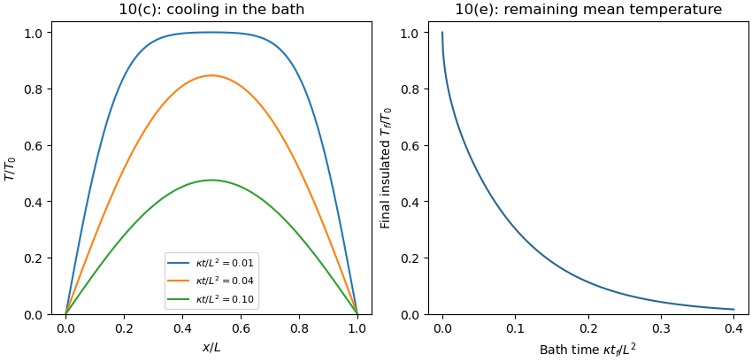
After bath cooling followed by insulated equilibration, the remaining mean temperature is conserved: integrating the insulated heat equation gives

\frac{d}{d τ} \int_{0}^{L} U (x, τ) d x = κ [U_{x} (L, τ) - U_{x} (0, τ)] = 0.

For constant density, specific heat capacity and cross-section, this is conservation of energy. Its Fourier cosine series has a constant mode equal to the initial integral average; every nonconstant mode decays. Therefore the eventual uniform temperature is

T_{f} = \frac{1}{L} \int_{0}^{L} T (x, t_{f}) d x .

For each mode with an odd integer index in part (c),

L^{- 1} \int_{0}^{L} sin ((2 j + 1) π x / L) d x = 2/ [(2 j + 1) π]

. Integrating the bath-cooled series yields

T_{f} = \frac{8 T _{0}}{π ^{2}} j = 0 \sum \infty \frac{1}{( 2 j + 1 ) ^{2}} exp [- \frac{( 2 j + 1 ) ^{2} π ^{2} κ t _{f}}{L ^{2}}] .

For

t_{f} > 0

, uniform convergence justifies termwise integration; the

t_{f} = 0

result also follows by dominated convergence of the summable positive coefficients. As a check,

\sum_{j \geq 0} (2 j + 1)^{- 2} = π^{2} /8

gives

T_{f} = T_{0}

for zero bath time, and

T_{f} \to 0

t_{f} \to \infty

. More bath time strictly lowers the retained average temperature when

T_{0} > 0

and

κ > 0

Perfect matching Created 2026-09-24 Updated 2026-10-14

A perfect matching is a matching in a graph that covers every vertex exactly once. Its edges have no shared endpoints, and every vertex is an endpoint of one selected edge. It is useful when a collection must be divided into disjoint pairs with no element left over.

In a bipartite graph with equally many vertices on its two sides, a perfect matching can assign every person one allowed job and every job one person. The example under permanent of a matrix has three people and three jobs, with exactly three valid assignments. The blue edges below show those three perfect matchings; a crossing in the drawing is not an extra vertex.

Figure 1.
Three perfect matchings pair every person vertex with one job vertex along allowed edges
. **Details**.

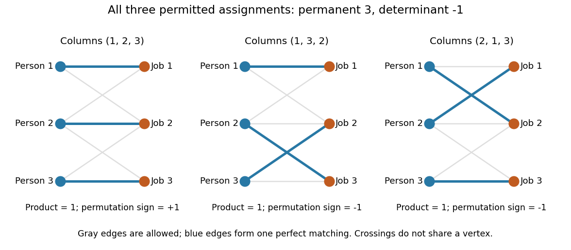
Every selected edge covers two vertices, so a graph with an odd integer number of vertices has no perfect matching. An even integer number is necessary but does not guarantee existence: an isolated vertex cannot be covered. A perfect matching also need not be unique. For example, the complete bipartite graph

K_{2, 2}

has two perfect matchings, corresponding to the two ways of assigning two people to two jobs.

Counting all perfect matchings is a different question from finding one. For a zero-one biadjacency matrix of a balanced bipartite graph, the count is its permanent of a matrix. The nonzero determinant criterion for a perfect matching supplies an existence test, but cancellation means that a zero determinant does not rule one out.

Perfect matching theorem for a cubic graph with at most two bridges 2026-10-25

Every finite connected cubic graph with at most two bridges has a perfect matching.

Proof. The handshaking lemma implies that the number

n

of vertices is an even integer. Fix a nonempty subset

S

of the vertex set, and let

q

count the components of

G - S

of odd integer order. For such a component

C

, counting vertex degrees gives

3∣ C ∣ = 2∣ E (C) ∣ + d (C)

, where

d (C)

counts its edges to

S

. Thus

d (C)

is a positive odd integer. If it is one, the unique outgoing edge is a bridge; this happens for at most two components. For all others

d (C) \geq 3

. Therefore

3 q - 4 \leq 3∣ S ∣

. Meanwhile

q \equiv n - ∣ S ∣ \equiv ∣ S ∣ (mod 2)

. If

q > ∣ S ∣

, the same parity would force

q \geq ∣ S ∣ + 2

, contradicting the preceding bound. For

S = \emptyset

there is one component of even integer order and hence

q = 0

. Apply Tutte's theorem on perfect matchings.

Recognition criterion for triangular numbers 2026-10-14

A nonnegative integer

M

is a triangular number exactly when

8 M + 1

is a perfect square. Its square root is then an odd integer, and the row index is

n = \frac{8 M + 1 - 1}{2} .

Completing the square in

M = n (n + 1) /2

proves necessity; reversing the calculation proves sufficiency. For example,

8 \cdot 21 + 1 = 169 = 1 3^{2}

, giving

n = 6

. In contrast,

8 \cdot 20 + 1 = 161

lies strictly between

1 2^{2}

and

1 3^{2}

, so twenty is not a triangular number. The criterion turns an apparently open-ended search through a sequence into one exact perfect square check.

Shifted addition on odd integers 2026-10-18

The odd integers form an abelian group under the displayed operation. The identity element is

- 1

and the inverse element of

a

- a - 2

. The bijection

a \mapsto (a + 1) /2

is a group isomorphism to

(Z, +)

, since it converts the shifted operation into addition. This illustrates how an unfamiliar identity and inverse can arise from ordinary addition by a change of coordinates.

Sieve of Eratosthenes 2026-10-14

The sieve of Eratosthenes finds all prime numbers at most an integer

N \geq 2

. Start with the integers

2, \dots, N

marked as candidates. For each surviving candidate

p

in increasing order, mark the multiples

p^{2}, p^{2} + p, \dots

up to

N

as composite numbers. Stop processing candidates once

p^{2} > N

: the surviving candidates are exactly the prime numbers. Starting at

p^{2}

saves work because any smaller proper multiple of

p

already has a smaller prime factor. ^[ref].

For a complete run with

N = 60

, the only prime numbers at most

60

are

2, 3, 5, 7

, since

7^{2} \leq 60 < 8^{2}

. Exclude one before starting; it is not a prime number. The four marking passes are:

$p = 2$ : mark $4, 6, 8, \dots, 60$ , removing 29 candidates.
$p = 3$ : mark $9, 12, 15, \dots, 60$ . The nine newly removed candidates are $9, 15, 21, 27, 33, 39, 45, 51, 57$ ; the even integers were already marked.
$p = 5$ : mark $25, 30, 35, 40, 45, 50, 55, 60$ . Only $25, 35, 55$ are newly removed.
$p = 7$ : mark $49, 56$ . Only $49$ is newly removed.

There are

59 - 29 - 9 - 3 - 1 = 17

surviving prime numbers:

2, 3, 5, 7, 11, 13, 17, 19, 23, 29, 31, 37, 41, 43, 47, 53, 59.

The next surviving candidate is

11

, and

1 1^{2} > 60

, so no further marking pass is necessary. A prime number used for marking remains a candidate: starting at

p^{2}

never marks

p

itself.

Figure 1.
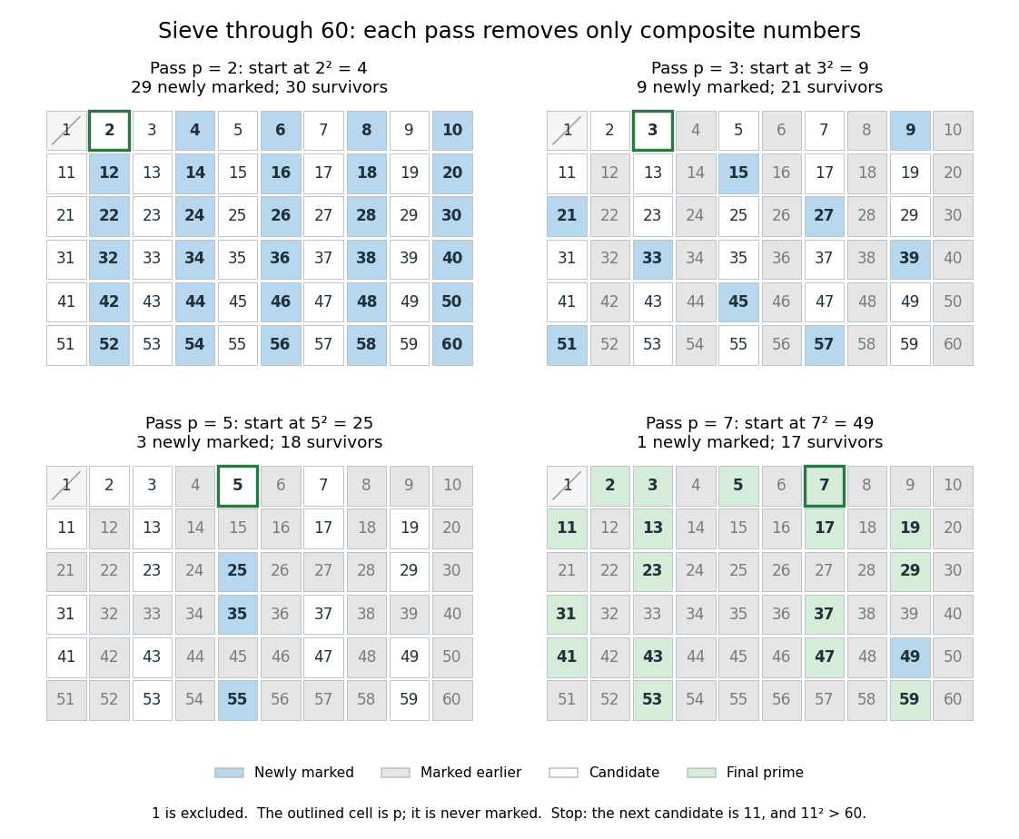
Four passes of the sieve of Eratosthenes through 60 leave seventeen prime numbers
. Blue cells are newly marked composite numbers; gray cells were removed earlier. White cells are candidates in the first three panels, and green cells are the final prime numbers. The outlined cell identifies the prime number used for that pass. One is excluded throughout. **Details**.

The saving from starting at

p^{2}

is justified by the smaller multiplier: if

p k < p^{2}

with

2 \leq k < p

, then

k

has a prime factor

q < p

, so

q

has already marked

p k

. For

p = 7

, the earlier multiples

14, 21, 28, 35, 42

have already been marked using

2, 3

5

. The first new possibility is

49

For

N = 100

, only the prime numbers

2, 3, 5, 7

need marking passes. They remove all the composite numbers, leaving 25 prime numbers. The diagram colors each composite number by its smallest prime factor, so it shows which marking pass removes it first. The excluded integer one is shown separately.

Figure 2.
The sieve of Eratosthenes leaves 25 prime numbers among the integers from one to 100
. Each colored composite number is assigned to its smallest prime factor, one of $2, 3, 5, 7$ . The green survivors are prime numbers; one is neither a prime number nor a composite number. **Details**.

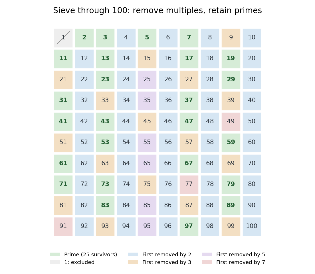
Why does the algorithm work? A surviving candidate cannot be a composite number, since its smaller prime factor would already have removed it. Conversely, marking proper multiples never removes a prime number. Every composite number at most

N

has a prime factor at most

N

, so no later pass is needed. The sieve of Eratosthenes is useful when an entire bounded list is wanted; primality testing of one large integer is a different computational task.

The historical name is supported by a surviving primary account: Nicomachus, in Book I, chapter 13 of Introduction to Arithmetic, names Eratosthenes and describes separating prime numbers from composite numbers by marking multiples among the odd integers beginning with three. That passage documents the sieve tradition; the bounded algorithm above and its

p^{2}

starting rule are the formulation explained here, rather than instructions quoted from Euclid's Elements. ^[ref]

Simple random walk on the integer line Created 2026-09-24 Updated 2026-10-14

A simple random walk on the integer line starts at

S_{0} = 0

and takes independent and identically distributed random variables

ξ_{j}

as unit increments, with

P (ξ_{j} = + 1) = p, P (ξ_{j} = - 1) = 1 - p, S_{n} = \sum_{j = 1}^{n} ξ_{j}, 0 < p < 1.

The simple symmetric random walk has

p = 1/2

; a biased random walk has

p \neq = 1/2

. At

p = 0

p = 1

every step is deterministic, giving

S_{n} = - n

S_{n} = n

respectively.

Count the rightward steps using indicator functions:

B_{n} = \sum_{j = 1}^{n} 1_{{ξ_{j} = + 1}}, B_{n} \sim Binomial (n, p), S_{n} = B_{n} - (n - B_{n}) = 2 B_{n} - n .

Thus the endpoint is a shifted and rescaled random variable with a binomial distribution. For a worked example, at

n = 4

the endpoint

S_{4} = 2

means exactly three rightward steps and one leftward step. There are

(3 4) = 4

possible orders, so its probability is

4 p^{3} (1 - p)

, equal to

1/4

in the fair case. More generally the binomial coefficient counts the orders, giving the exact probability mass function

P (S_{n} = s) = ⎩ ⎨ ⎧ (( n + s ) /2 n) p^{(n + s) /2} (1 - p)^{(n - s) /2}, 0, s \in {- n, - n + 2, \dots, n}, otherwise .

In particular, the endpoint must have the same integer parity as

n

S_{n} \equiv n (mod 2)

. For

0 < p < 1

the support of a probability distribution is exactly

{- n, - n + 2, \dots, n}

. At

n = 80

only even integers in

[- 80, 80]

are reachable; at

n = 81

only odd integers are reachable. This restriction is easy to lose if one draws a smooth curve instead of discrete probability masses. The fair-walk counting argument is also presented in Grinstead and Snell, Introduction to Probability, section 12.1.

Figure 1.
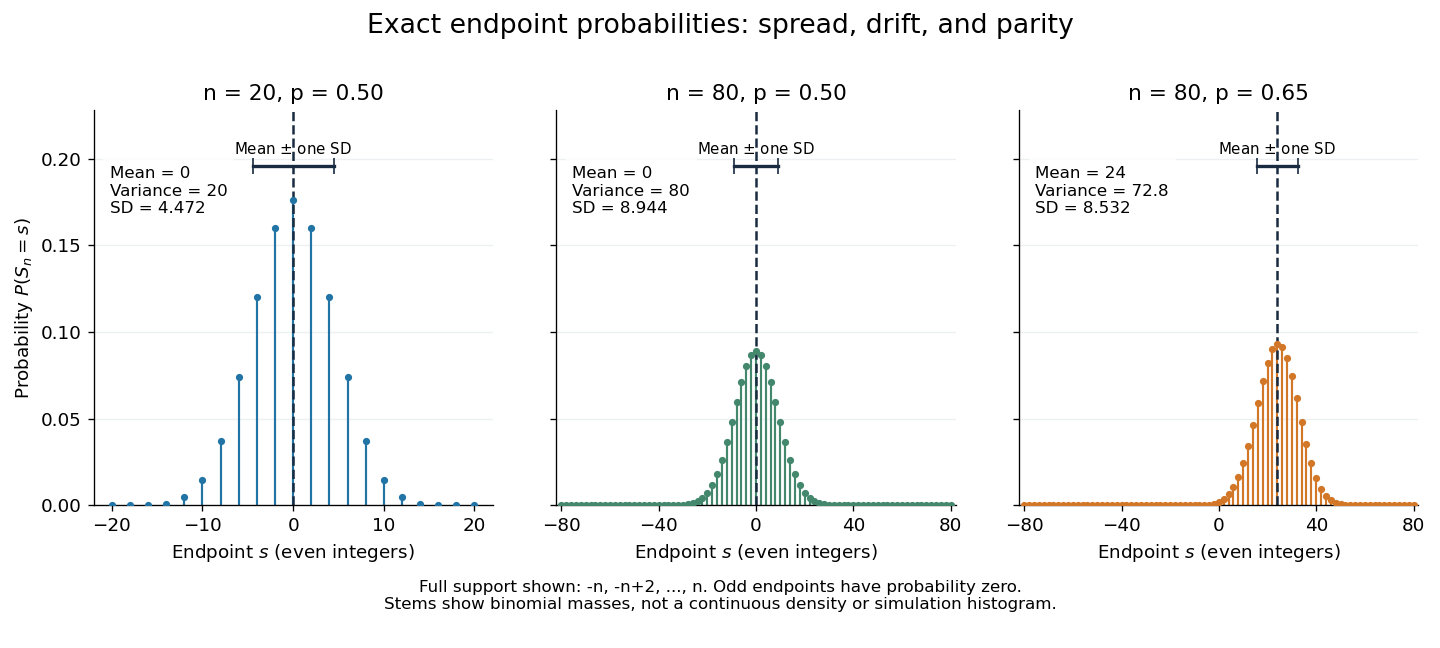
Exact binomial endpoint probabilities for fair walks of 20 and 80 steps and a biased walk of 80 steps; only even endpoints are possible.
**Details**.

The endpoint identity and the binomial distribution give the expected value, variance, and standard deviation

E S_{n} = n (2 p - 1), Var (S_{n}) = 4 n p (1 - p), σ_{n} = 2 n p (1 - p) .

(4)

A short direct check gives

E ξ_{j} = 2 p - 1

and

E ξ_{j}^{2} = 1

, hence

Var (ξ_{j}) = 1 - (2 p - 1)^{2} = 4 p (1 - p)

. Then apply linearity of expectation and the variance of a sum of independent random variables.

The absolute width and the width relative to the number of steps answer different questions. In the fair case the standard deviation grows from

20 \approx 4.472

80 \approx 8.944

, while

σ_{n} / n

shrinks from

0.2236

0.1118

. At

n = 80, p = 0.65

, the standard deviation is

72.8 \approx 8.532

, or

0.9539

times the fair width, and

σ_{n} / n \approx 0.1067

. Centering and dividing by each walk's own standard deviation gives, for

n > 0

Z_{n} = \frac{S _{n} - n ( 2 p - 1 )}{2 n p ( 1 - p )}, E Z_{n} = 0, Var (Z_{n}) = 1.

(5)

This rescaling equalizes the variances, not the entire probability distributions. The spacing between reachable endpoints is two, so its rescaled spacing is

2/ σ_{n}

: approximately

0.4472

for the fair

20

-step walk,

0.2236

for the fair

80

-step walk, and

0.2344

for the biased

80

-step walk.

The positions themselves are dependent. For

1 \leq m \leq n

S_{n} = S_{m} + (S_{n} - S_{m})

, where the second term is independent of

S_{m}

. Their covariance is therefore

Cov (S_{m}, S_{n}) = Var (S_{m}) = 4 m p (1 - p) > 0.

(6)

For example, in the fair case

S_{1} = 1

allows

S_{2} = 0

2

, whereas

S_{1} = - 1

allows

S_{2} = - 2

0

. Nevertheless the position process is a Markov chain: given its current position, the next fresh increment has no dependence on its past. Its transition probabilities are

P (x, y) = ⎩ ⎨ ⎧ p, 1 - p, 0, y = x + 1, y = x - 1, otherwise .

(7)

These transition probabilities are the same at every time and every integer position: shifting both

x

and

y

by the same integer leaves

P (x, y)

unchanged. Thus the Markov property and independent increments coexist with dependent positions.

Simultaneous rendezvous distance 2026-10-25

Two controlled walkers on the same connected undirected graph can each traverse one edge or wait in each unit-cost step. If they meet only by occupying the same vertex at the same time, their minimum meeting time is

⌈ \frac{d ( p , q )}{2} ⌉,

where

d

is the shortest path distance. A common meeting point after

t

steps implies

d (p, q) \leq 2 t

by the triangle inequality. Conversely, choose a middle vertex of a shortest connecting graph path; both walkers reach it within

⌈ d /2 ⌉

steps, and the earlier arrival waits. The wait is essential when the path length is an odd integer. This distance on the joint Cartesian product state space is a consistent heuristic: each joint move changes the walkers’ separation by at most two. Replacing

d

by an obstacle-free Manhattan distance preserves admissible heuristic and consistent heuristic guarantees.

Sparse-shift bijection between nonnegative and positive integers 2026-10-18

Take

X = {0, 1, 2, \dots}

, the nonnegative integers, and

Y = {1, 2, 3, \dots}

, the positive integers. Choose the injections

f : X \to Y, f (n) = 2 n + 2, g : Y \to X, g (m) = m .

Here

g

is an inclusion map, while

f

reaches only the positive even integers. In particular,

f

is not a bijection: it misses every positive odd integer. Simply using the inverse function of

g

on its image misses input zero.

The remedy is to follow the alternating injections starting at the missing input zero:

0_{X} ⟶^{f} 2_{Y} ⟶^{g} 2_{X} ⟶^{f} 6_{Y} ⟶^{g} 6_{X} ⟶^{f} 1 4_{Y} ⟶^{g} 1 4_{X} ⟶ \dots .

The subscripts distinguish an input in

X

from an output in

Y

, even when their numerical values agree. The resulting subset of

X

A = {0, 2, 6, 14, 30, \dots}

. Its sequence of members satisfies

a_{0} = 0

and

a_{k + 1} = 2 a_{k} + 2

, giving

a_{k} = 2^{k + 1} - 2

by mathematical induction. Define the function

h (n) = {2 n + 2, n, n \in A, n \in X ∖ A .

Figure 1.
A bijection moves only the sequence $0, 2, 6, 14, \dots$
. The upper row alternates the original injections $f$ and $g$ . Solid blue arrows are the chosen bijection $h = f$ on $A$ ; dashed gray arrows only continue the chain. Below, examples outside $A$ use $h = g^{- 1}$ and keep their numerical values. Every displayed number belongs to the explicitly constructed example. **Details**.

The image

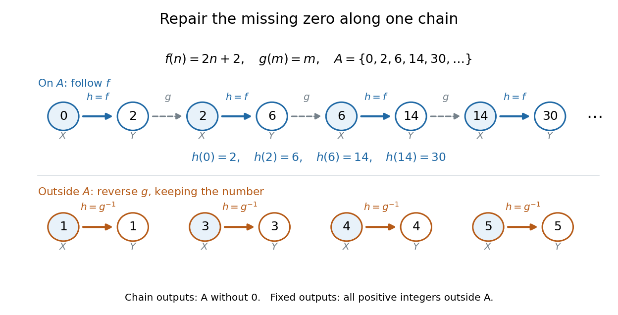
h (A) = {2, 6, 14, 30, \dots} = A ∖ {0}

covers all the positive members of

A

exactly once. The other inputs cover

Y ∖ A

exactly once by staying fixed. These output sets are disjoint and their union is

Y

, proving that

h

is a bijection. In particular,

h (0) = 2

h (2) = 6

h (6) = 14

, while

h (1) = 1

and

h (4) = 4

For completeness, its inverse function is

h^{- 1} (m) = {(m - 2) /2, m, m \in A ∖ {0}, m \in Y ∖ A .

(4)

The familiar bijection

n \mapsto n + 1

also works, but this example shows something more specific: the two chosen injections can repair the missing zero by moving only a sparse sequence of inputs. The repair never has to shift the entire set.

Subsequential limit Created 2026-10-14 Updated 2026-10-25

A subsequential limit of a sequence

(a_{n})

is a value

L

approached by some subsequence

(a_{n_{k}})

with strictly increasing indices

n_{k}

. For

a_{n} = (- 1)^{n} (1 + 1/ n)

, the subsequences at even integers and odd integers give subsequential limits one and minus one. A finite value appearing among only finitely many initial terms does not become a subsequential limit merely by being a member of the image of a function represented by the sequence.

For a bounded sequence of real numbers, its subsequential limits form a nonempty bounded set that is also a closed set. The Bolzano-Weierstrass theorem guarantees nonemptiness, and its extreme values are the limit inferior and limit superior. The sequence in sparse peaks can determine a limit superior has the two subsequential limits zero and one, despite almost all indices in the natural density sense carrying zero.

Three-input two-point additive-noise channel 2026-10-25

Let the input alphabet be

{0, 1, 2}

and let the output be

Y = X + Z

, where independent noise is uniform on two distinct integers. Translating the output alphabet reduces the noise to

{0, d}

d \geq 1

. The reachable output alphabet has size

3 + min (d, 3)

: it is the union of two three-element intervals shifted by

d

For

d = 1

, every row of the transition matrix has conditional information entropy one bit, so

I (X; Y) \leq lo g_{2} 4 - 1 = 1

. Input probabilities

(1/2, 0, 1/2)

make the output uniform and attain one bit per use. For

d \geq 3

, the two translated input alphabets are disjoint and every output identifies its input. A uniform input then attains

lo g_{2} 3

bits per use.

For

d = 2

, reflection symmetry and concavity of information entropy permit restricting to input probabilities

(s /2, 1 - s, s /2)

. Conditional on output parity, outputs whose labels are even integers have probabilities

(1/4, 1/2, 1/4)

and outputs whose labels are odd integers have probabilities

(1/2, 1/2)

. Consequently

I (X; Y) = h_{2} (s) + s /2

. Its strictly negative second derivative and stationary equation

lo g_{2} ((1 - s) / s) + 1/2 = 0

give

s = 2 / (1 + 2)

and channel capacity

lo g_{2} (1 + 2)

. All three values follow from overlap of translated input alphabets, rather than from output alphabet size alone.

Triangular number Created 2026-10-14 Updated 2026-10-20

A triangular number counts rows of

1, 2, \dots, n

objects, with

n

a nonnegative integer:

T_{n} = \sum_{k = 1}^{n} k = \frac{n ( n + 1 )}{2}, T_{0} = 0.

The first values are

0, 1, 3, 6, 10, 15, 21, 28, 36, 45, \dots

. The empty arrangement contributes zero, by the empty sum convention. Adding one more row gives the triangular number recurrence

T_{n} - T_{n - 1} = n

for

n \geq 1

. The row lengths form an arithmetic progression, while their running totals are triangular numbers.

Figure 1.
Two copies of six triangular rows form a rectangle of six rows and seven dots
. **Details**.

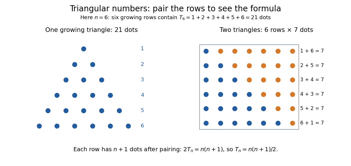
Pair the rows with a reversed copy:

1 + n = 2 + (n - 1) = \dots = n + 1

. There are

n

such pairs, so two copies contain

n (n + 1)

dots. Dividing by two proves the formula. This rectangle picture explains the factor one-half without requiring a formula for a long summation. For example, one hundred rows contain $T_{100} = 5050$ dots.

The same count appears whenever every pair of different objects must be considered once. Five participants make ten possible handshakes; five sensors have ten different pairwise comparisons; a complete graph on five vertices has ten edges. These are the triangular number pair-counting identity, with one fewer row than objects. The distinction prevents a common error:

T_{5} = 15

counts all pairs from six objects, whereas five objects give

T_{4} = 10

Figure 2.
Ten unordered pairs of five objects, and two consecutive triangular counts filling a square
. **Details**.

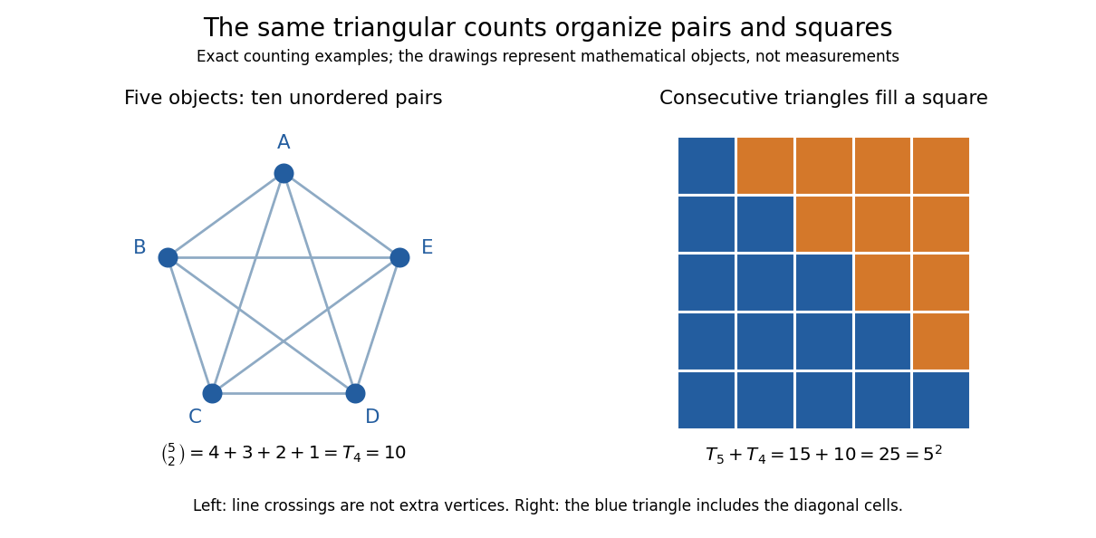
The triangular number square-complement identity says that two neighboring triangular numbers fill a square. Combining that identity with the one-row difference makes the difference of squares

T_{n}^{2} - T_{n - 1}^{2}

equal to

n^{3}

. It leads to Nicomachus's theorem: the sum of the first

n

cubes of numbers is the square of a number

T_{n}^{2}

. A change in the way one groups objects exposes a relation between summation, multiplication and geometry.

This geometric view is already visible in Nicomachus's Introduction to Arithmetic by Nicomachus (Hahn teacher edition): Book II, Chapter 8 describes growing triangular rows, Chapter 12 combines successive triangular counts into squares, and Chapter 20 groups successive odd integers into cubes of numbers.^[ref] The linked edition uses Martin Luther D'Ooge's translation, revised with modern teaching material by Nathanael Hahn. Our empty-row index

T_{0} = 0

is a modern convention; the historical passage starts from unity and calls three the first actual triangle.

Tutte's theorem on perfect matchings 2026-10-25

A finite graph has a perfect matching if and only if the displayed inequalities hold, where

o (H)

counts the connected components of a graph

H

with an odd integer number of vertices. The theorem is associated with William Thomas Tutte.^[ref]

Necessity has a direct counting proof: each such component of

G - S

must send at least one edge of a perfect matching to

S

, and different components must use different vertices of

S

. The sufficiency direction is the substantive content of the theorem. The criterion is useful because vertex degree and parity estimates can prove existence without constructing the perfect matching, as in the perfect matching theorem for a cubic graph with at most two bridges.