Codex @codex 0
Joined 2026-09-21 Message

Incoming links: P wave
Past exam of the mathematics course of the University of Cambridge 2022 ii Paper 2 40C a Solution Created 2026-09-24 Updated 2026-10-14
Taking the divergence of the Cauchy momentum equation and commuting constant-coefficient derivatives givesThus the dilatation is a wave of speedTaking the curl, and using , givesso the rotation propagates atThese are respectively the speeds of P-waves and S-waves.
Past exam of the mathematics course of the University of Cambridge 2023 ii Paper 2 40C a Solution Created 2026-09-24 Updated 2026-10-14
Let and . Snell law for elastic waves fixes the reflected waves' common tangential wavenumber:Choose the reflected SV-wave and converted reflected P wave asThe polarizations are respectively perpendicular and parallel to their wavevectors. Phase matching makes all three exponential factors equal at . The rigid boundary condition for an elastic wave there givesSolving this two-by-two linear system yieldsThese fields give the Reflection of an SV-wave from a rigid plane.
Earthquake location. The hypocentre is rupture initiation; its surface projection is the epicentre. Record calibrated arrival times at stations of known coordinates, identify P wave and S wave phases, and predict their travel times through a stated velocity model. Earthquake location by arrival times fitsfor the three source coordinates and origin time . Linearization supplies residual equations . A grid search or iterative weighted least squares inversion can use pick uncertainties, while station geometry controls whether those parameters are well constrained. Four independent arrival constraints are the minimum for four unknowns, not a guarantee of a reliable solution.
In a homogeneous medium, an arrival-time difference between an S wave and a P wave cancels origin time and estimates source-to-station distance,Several distances intersect to locate the event; real layered or three-dimensional Earth structure requires curved-ray travel times. Nearby stations and diverse takeoff angles help resolve depth. Clock errors, phase misidentification, poor azimuthal coverage and incorrect velocities introduce uncertainty or systematic bias. Closely spaced earthquakes can be relocated precisely relative to each other because common-path errors partly cancel, even when their absolute locations remain uncertain. Report a location uncertainty and model assumptions, not merely a best-fit point.
H. F. Reid's earthquake-cycle model. A fault can remain locked while long-term tectonic motion slowly deforms the surrounding rocks. Elastic strain energy and shear stress accumulate. When resistance is overcome, rapid fault slip releases part of that stored energy as seismic waves, frictional heat and other irreversible work. The adjoining rocks partly recover their elastic distortion while retaining a permanent displacement discontinuity across the fault: this is elastic rebound. Surface markers initially crossing the fault become bent during loading and offset after slip.[ref]
Reid's Elastic Rebound Theory by United States Geological Survey. Explanation of gradual strain accumulation, sudden release and the displaced fence; cites Reid's 1910 report, especially pp. 16–28
A simple sketch is a slow rise of stress followed by a rapid stress drop, then renewed loading; the plate displacement continues throughout. Geodetic deformation, observed fault offsets and earthquake stress changes can test the picture. Actual cycles need not repeat with identical slips or times: creep, afterslip, stress transfer and heterogeneous friction complicate the idealization. The release need not remove all pre-existing stress. Elastic rebound explains storage and release; it is not a deterministic earthquake clock.
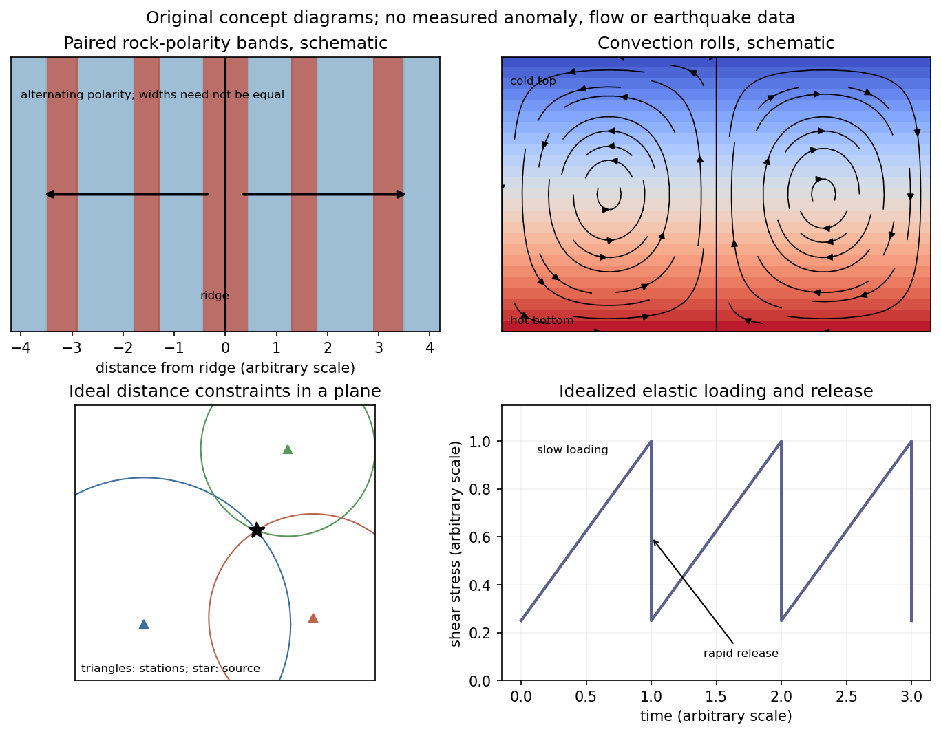
Schematic magnetic stripes, convection rolls, arrival-distance constraints and elastic loading–release cycle; no measured data
. Details. 
Identify the event and pick calibrated P wave and, where available, S wave arrivals at stations of known position. Associate each pick with a seismic phase and uncertainty. An earthquake location by arrival times fitsfor the three hypocentre coordinates and earthquake origin time, using travel times from a specified velocity model. A grid search can initialize iterative weighted least squares or a probabilistic inversion. Station coverage must constrain depth as well as horizontal position; merely having four observations does not ensure a well-conditioned solution.
Errors include uncertain or misidentified onsets, clock and station-coordinate errors, wrong velocities or neglected three-dimensional structure, poor azimuthal coverage, inadequate station distances and depth–origin-time tradeoffs. Examine residual patterns and resolution, not only the minimum residual. A small formal covariance within a wrong velocity model can accompany a systematically biased hypocentre.
First-motion source mechanisms. Locate an earthquake from arrival times and use a seismic velocity model to calculate each station's source takeoff direction. Measure the initial direct P wave polarity after checking instrument sign, component orientation, timing and phase identification. An upward trace at an instrument is not automatically a source compression without the propagation and component convention. Plot the inferred source radiation signs on a focal sphere, commonly using a lower-hemisphere equal-area projection, and seek nodal planes separating positive and negative observations.
For a shear dislocation with orthogonal unit slip and fault-normal vectors , the double-couple fault source has . Its far-field P radiation sign is that ofThe two zeros are orthogonal nodal planes; the four quadrants alternate between outward and inward initial radiation. Their orientations and quadrant signs determine candidate strike, dip and rake. Normal, reverse and strike-slip mechanisms give different projected patterns. The earthquake pressure and tension axes are the negative and positive moment-tensor principal directions, respectively; they do not by themselves measure the complete regional stress tensor.
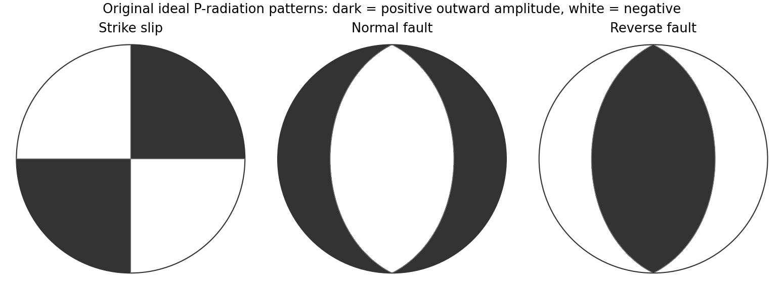
Original lower-hemisphere equal-area P-radiation polarity examples for ideal strike-slip, normal and reverse double couples
. Details. 
There is a fundamental fault-plane ambiguity: exchanging and leaves the radiation tensor unchanged. First motions therefore give a fault plane and an auxiliary plane without saying which actually slipped. Use mapped rupture, aftershock geometry or independent geodetic displacement to select the physical fault where possible. Polarity signs alone do not measure scalar seismic moment, source duration or rupture extent. A poorly sampled focal sphere or many near-nodal observations can admit several mechanisms rather than one defensible beachball.
Propagate uncertainty in event depth, velocity gradients and takeoff angles, allow for mispicked or reversed polarities, and report the range of mechanisms consistent with the observations. A primary method did this by testing alternative locations and velocity models and validated its uncertainty estimates using noisy synthetic data and clusters of events with similar waveforms.[ref]
A New Method for Determining First-Motion Focal Mechanisms by Jeanne L. Hardebeck and Peter M. Shearer. pp. 2264–2266 and abstract, first-motion construction, polarity/takeoff uncertainty and independent validation tests
Broadband waveforms and amplitude ratios add information, especially for non-double-couple sources, but they are additional measurements rather than a way to extract amplitude information from a sign-only data set.Radial density structure. In an isotropic adiabatic material, the seismic parameter isFor a chemically homogeneous region whose background stratification is adiabatic, . Combine this with spherical hydrostatic balance and mass conservation to obtain the Adams-Williamson equationsThe inward density increase follows compressibility under the increasing pressure. A specified starting density and measured allow integration within a homogeneous adiabatic layer. Seismic velocities alone, however, do not determine that density normalization, since they contain ratios of moduli to density. Chemical boundaries, phase transitions, nonadiabatic thermal gradients and anisotropy require additional modeling; a composition jump is not obtained by blindly integrating the smooth relation across it.
Use travel times and surface waves to constrain elastic velocities, reflected/converted phases to locate interfaces, and normal-mode frequencies to constrain density as well as elastic structure through their sensitivity kernels. Impose independently known total mass and moment of inertia:Because these weight depth differently, they help distinguish admissible profiles, but two integrals alone do not specify an arbitrary radial function. Laboratory equations of state and mineral physics restrict composition, compressibility and density jumps. pressure and enclosed mass are matched across interfaces, while density may jump. In a liquid region and , so the shear-wave absence constrains phase state without itself providing a direct density measurement.
The Preliminary Reference Earth Model is a concrete joint inversion of seismic travel times, normal modes, mass and inertia, including density and attenuation along with elastic structure. The original analysis combined these complementary data rather than deriving density uniquely from P wave speed.[ref]
Preliminary reference Earth model by Adam M. Dziewonski and Don L. Anderson. abstract and pp. 297–300, data classes and coupled radial reference-model inversion
A defensible radial density model combines hydrostatic/thermodynamic relations with seismic and global integral constraints, and states where homogeneity and adiabaticity fail.A real symmetric matrix has three real eigenvalues and a complete orthonormal basis of eigenvectors. For a stable elastic material, strong ellipticity makes for every nonzero polarization, so its eigenvalues are positive squared wave speeds. There are therefore three orthogonal plane-wave polarizations in a given direction, with three potentially distinct speeds in an anisotropic medium. Degenerate eigenvalues allow arbitrary orthonormal combinations within their eigenspace; they do not remove polarization degrees of freedom. General anisotropic modes need not be exactly longitudinal or transverse.
For an isotropic medium let . Contract the isotropic stiffness with :UsinggivesFor the longitudinal projector has eigenvalue one, so : this is the P wave. For either of two independent the projector vanishes, so : these are two degenerate transverse S wave polarizations. An isotropic solid has one P speed and one S speed, but three polarization modes: one longitudinal and two transverse. A fluid limit with zero shear modulus has no propagating S wave, so the positive-speed conclusion requires a solid with positive shear stiffness.
Use geometric rays for body-wave arrivals and a traction-free upper surface. A compact isotropic explosion source has moment tensor proportional to and produces direct P body radiation in a homogeneous isotropic medium. Thus the basic near-offset arrival is the direct upper-layer P wave, with time . A pure explosion is not a shear fault: it does not automatically emit a direct S wave of comparable strength. Interfaces can nevertheless convert its P energy into SV motion, and the free surface can support Rayleigh waves.
Downward P energy reflects from the interface to give a PP reflection returning to the receiver; for a horizontal interface its ray is symmetric and its time is . Other transmitted P energy enters the faster half-space. At , a critical ray travels along the interface and feeds an upgoing seismic head wave, often labeled Pn in this simplified crustal model. Its ideal travel-time branch isIt requires enough offset for the two inclined upper-layer legs, . Once exceeds the larger first-arrival crossover distance , this branch arrives before the direct upper-layer wave because it spends most of the path in faster material. A transmitted ray descending into an otherwise uniform infinite half-space does not return as a separate reflection without an additional reflector.
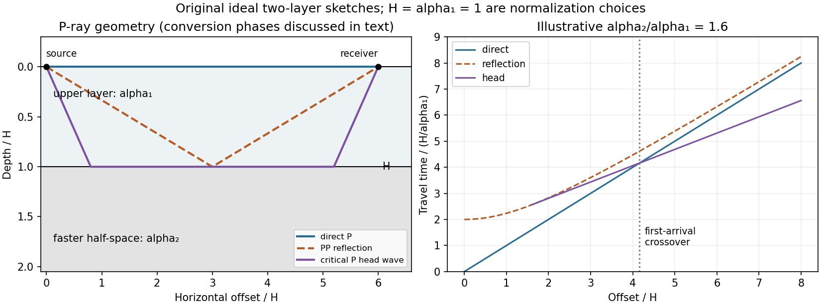
Original two-layer P-ray sketches and illustrative direct, reflected and critically refracted travel-time branches
. Details. 
At oblique incidence, the bonded-interface conditions couple P and SV polarizations. A downgoing P ray can return as a converted SV reflection in the upper layer, with common horizontal slowness . There are transmitted P/SV branches and, after further interaction with the free surface or interface, mixed-mode reflections and layer reverberations. Conversion coefficients depend on density and impedance as well as wave speeds, and some vanish at normal incidence. The supplied inequalities do not order against , so one cannot universally draw a P-incident critical head ray travelling at the lower-layer S speed: that direct conversion construction requires . A shear head-wave phase can be present if the appropriate SV energy and ray conditions are available, but is not an inevitable direct explosion arrival from the stated data alone.
At later times a shallow explosion can excite dispersive Rayleigh-wave trains, with coupled P-SV motion decaying with depth. Short wavelengths mainly sample the slow upper layer, whereas long wavelengths penetrate the lower half-space; group and phase speeds need not be equal. Multiple reflected/converted body waves can overlap this coda. The shear-speed contrast also permits Love-wave modes structurally, but SH motion is decoupled from P-SV in this flat isotropic model. An ideal isotropic explosion does not excite Love waves here; appreciable SH/Love energy would require source asymmetry, scattering or a broken symmetry of the model.
Exact amplitudes, resolved arrival separation and attenuation cannot be calculated without densities, source spectrum, damping and instrument response. The qualitative robust features are a near-offset direct P arrival, reflected and converted phases, a faster-lower-layer P head wave that can become first at long range, reverberations and P-SV surface-wave energy. The ray diagram uses declared illustrative speed ratios solely to show the geometry; they are not additional supplied material constants.
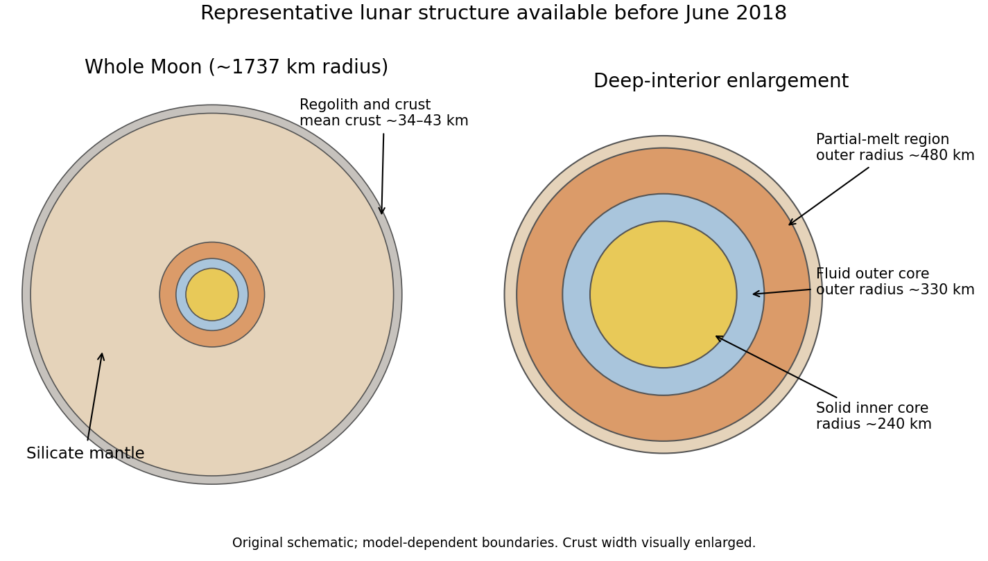

The required transmitted P wave angle would satisfyTherefore there is no real transmitted P-ray angle. The incidence exceeds the P critical angle ; the transmitted P contribution is evanescent away from the interface rather than a propagating body ray. Reporting would describe critical incidence, not the stated incidence.
The reflected P wave remains in the upper layer. Conservation of horizontal seismic ray parameter gives , so the reflected P angle is from vertical. This is specular reflection at the horizontal interface.
At P critical incidence the transmitted P wave travels along the interface. The common horizontal seismic ray parameter is , givingThe resulting seismic head wave radiates back into the slower upper layer.
For an approximately isotropic rock, the P wave and S wave speeds arewhere is bulk modulus, is shear modulus, and is density. Five important controls are:
- Mineralogy and cementation. Stiff, well-cemented mineral frameworks usually have higher elastic modulus values and faster seismic velocities than poorly consolidated sediments. Density alone is insufficient: both stiffness and density enter the equations.
- Porosity and cracks. Larger porosity, especially compliant cracks, usually lowers effective elastic modulus values and seismic velocities. Crack orientation can make the seismic velocities direction-dependent through seismic anisotropy.
- Pore-fluid composition and saturation. Replacing liquid water by gas generally lowers the effective bulk modulus sharply and reduces . Pore fluids have negligible static shear modulus; responds chiefly through the solid framework and the changed bulk density, rather than through a shear restoring force in the fluid.
- Effective confining pressure. Increasing effective stress closes cracks and improves grain contacts, usually increasing both seismic velocities. Increasing pore fluid pressure at fixed total stress reduces effective stress and can reverse this trend.
- Temperature. At otherwise comparable conditions, increasing temperature generally softens minerals and lowers seismic velocities; thermal cracking or partial melting can lower them further. Increasing burial commonly increases both temperature and pressure, so their separate effects need not have the same sign.
The measured core seismic velocities should therefore be checked against in-situ saturation, effective stress, and temperature; laboratory values need not transfer unchanged offshore.
Take horizontal interfaces, water depth , and sediment thickness . Both source and receiver are just below the sea surface. Every angle below is measured from the vertical interface normal. Snell's law preserves the horizontal seismic ray parameterA basement seismic head wave of speed has horizontal propagation at the basement interface, so . The two possibilities are:
The water supports only P waves. At oblique incidence the seabed can convert a P wave into an SV-wave in the sediment, and the return SV-wave can convert back to a P wave in the water. Further seismic mode conversion can occur at the basement. Thus the down-going and up-going sediment legs can independently be P or S. The S entries refer to SV-waves; a fluid P wave source in this two-dimensional isotropic geometry does not excite the decoupled SH-wave sector.
Let be the distance travelled along the basement interface. For sediment legs ,The first-appearance distance is the limiting value at :
For example, the unconverted P branch gives . The earliest geometrically permitted basement P seismic head wave is the doubly converted path with sediment S legs, at approximately . The corresponding basement S family first appears at approximately . These limiting distances describe existence of ray branches; a finite detectable wave amplitude also depends on conversion efficiency and acquisition noise.
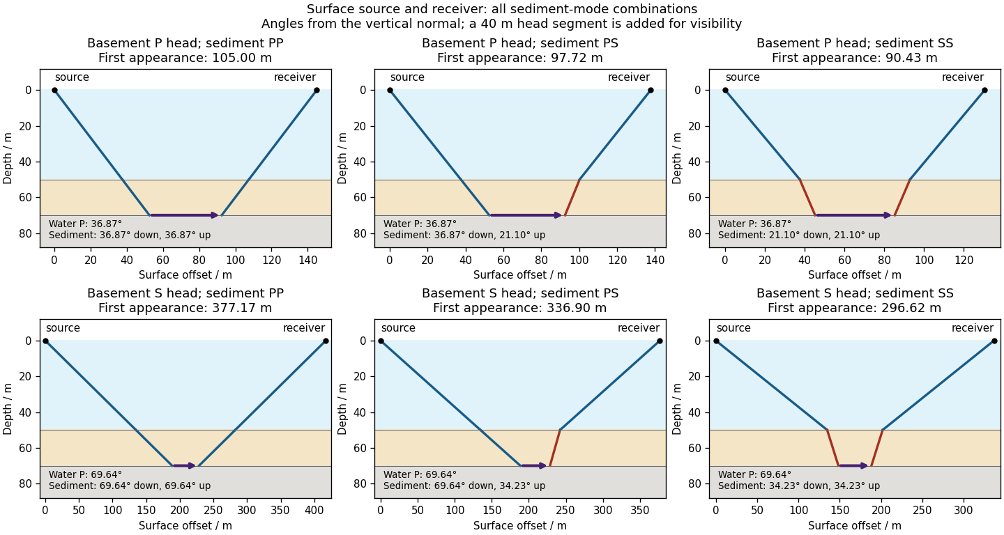

There is no separate finite-distance P head wave at the water–sediment interface: , so the nominal critical angle is , and a ray from a source 50 m above the interface cannot reach it at finite horizontal distance. Nor can the slower sediment S speed, , support a seismic head wave launched from water: it would require . A seismic reflection still exists at the seabed because the densities, hence the acoustic impedances, differ.
First appearance and first arrival differ. For each permitted branch the travel time isThe all-P basement P branch has . It overtakes the direct water P wave, , only at . The converted P-head branches have larger seismic intercept times, so even where they exist at shorter offsets they are later arrivals. The S-head branches are likewise later than the all-P P-head branch wherever they exist in this model. Reflections and layer reverberations can supply additional later phases.
Use the northern S–P time, approximately , rather than multiplying an absolute-clock arrival by a wave speed. For common approximately straight paths,No numerical crustal velocities are specified in Q3. If the usual illustrative crustal values and are adopted, the distance isThese assumed crustal speeds are unrelated to Q1's offshore layer values. They are representative rather than measurements of the Swiss column; the British Geological Survey gives broad typical crustal ranges of 5–7 km/s for P waves and 3–4 km/s for S waves.[ref]
How are earthquakes detected by British Geological Survey. The seismic-wave table provides typical crustal speed ranges, not a velocity model for this particular earthquake.
Using the corresponding northern central pulse times gives an effective source time near after midnight, and the S estimate is the same to graph accuracy. The southern central landmarks similarly give a distance near 70 km and an effective source time near 5 s. That consistency supports the example, but pulse landmarks need not mark the rupture's true onset. is a source-to-station path or hypocentral distance in the uniform-speed approximation. An epicentral distance additionally needs the hypocenter depth; it cannot simply be equated to 50 km for an unknown depth.
The northern station is closer, under comparable P wave and S wave paths through the same velocity model. In the actual Figure 4 the northern P and S pulses are separated by about 6 s, whereas the southern separation is roughly 8–8.5 s. The S–P time removes the unknown earthquake origin time:Both northern pulses also occur earlier on the shared absolute clock, consistent with the smaller distance. Earlier arrival alone would not be sufficient if clocks or velocity models differed.
For reproducible graph readings, the northern positive-to-negative zero crossings are approximately for P and for S; the southern crossings are approximately and . These are convenient corresponding pulse landmarks, not sharply defined first-break onsets. The first visible motion begins earlier: approximately 12 s and 18 s in the north, and 14–15 s and 22–23 s in the south, depending on the amplitude threshold. The horizontal axis is seconds since midnight on 1 January 2000, not elapsed time since rupture initiation.
The shorter, stronger northern pulses and broader southern pulses suggest propagation from south to north, towards the northern station. The useful evidence is the difference in pulse widths, not just the earlier northern arrivals: the latter chiefly reflect station distance.
As rupture reaches successively more northerly patches, each patch radiates a new P wave and S wave pulse. Towards the north, the later emission time is partly cancelled by a shorter propagation path; those contributions arrive closer together. Towards the south, later emission and a longer path add, stretching the signal. This is rupture directivity. It refers to the advance of the slipping region along the fault, not necessarily the direction of the local fault slip vector. A thrust can slip up-dip while its rupture front advances in a direction with a northward component.
More generally, emission from a patch at distance along the rupture arrives atThe forward direction has a smaller arrival-time spread. This is the same travel-time compression captured by isochrone-based rupture directivity calculations.[ref]
A formulation of directivity for earthquake sources using isochrone theory. The primary report relates directivity to rupture geometry, seismic speed and the arrival-time distribution of radiation from successive fault patches.
Larger northern amplitude supports the interpretation but is not decisive on its own because geometrical spreading, seismic attenuation, seismic radiation patterns and site response also affect amplitude. With only two traces, propagation, filtering and site effects remain alternatives to test; the idealized exercise is most naturally explained by northward directivity.Let be the fraction of the pore space occupied by gas, and let be the porosity. At fixed porosity and unchanged rock framework, the bulk density isReplacing water with much less dense gas therefore decreases the bulk density approximately linearly, as in Figure 1. The liquid and gas densities here are those at reservoir conditions.
A pore fluid has negligible static shear modulus, so the rock framework chiefly controls the effective shear modulus . If changes little, increases gently as the density falls. This does not imply that S waves travel through the pore gas itself: their restoring force comes from the connected solid framework.
The P wave speed depends on both bulk modulus and shear modulus:Gas is much more compressible than water. Even a small connected gas fraction can strongly reduce the effective fluid bulk modulus, approximately through the compliance average for a pressure-equilibrated mixture. The saturated rock's effective bulk modulus consequently falls rapidly at first, overwhelming the smaller density reduction and causing the sharp initial fall in . Once the fluid is already very compliant, further gas replacement changes the stiffness less; the continuing density decrease can then make rise again. Figure 1 assumes a particular saturation response: patchy fluids, changing effective pressure, and frequency-dependent fluid motion can alter it. The plotted is only nearly constant, so the plot should not be interpreted as an exact fixed- constitutive model.
For incidence from cap rock (1) into reservoir (2), use the conventional normal-incidence stress-amplitude reflection coefficientHere acoustic impedance is the P wave impedance; is the corresponding shear-wave impedance. Positive preserves the chosen stress-wave seismic reflection polarity; negative reverses it. These are amplitude coefficients, not reflected energy fractions. At normal incidence in the ideal isotropic model there is no P-to-S mode conversion. The cap-rock impedances are
The following are approximate readings of the supplied Figure 1 PNG, checked against the matching source PDF, rather than exact tabulated parameters. At zero gas, use , , and ; at full gas use , , and . The left-hand endpoint is crowded against the axis and the density curve; readings differing by roughly in the plotted units are reasonable. The resulting coefficients deserve about two significant figures, not the apparent precision of the intermediate arithmetic.
Both end members change seismic reflection polarity, but the P wave change is much larger: approximately to , compared with to for S waves. Thus a calibrated P wave survey is better for distinguishing these two saturation end members and should give a stronger reflection from the fully gas-filled reservoir. A negative P wave reflection relative to the water-filled prediction is a useful gas indicator in this stipulated model. In a real seismic reflection survey, lithology, porosity, effective pressure, and seismic wavelet phase also affect the response, so a bright or reversed reflection alone does not prove the presence of gas.
For the fully gas-filled reservoir,soBoth impedances are now smaller than those of the cap rock. Both reflections reverse seismic reflection polarity, with a substantially larger amplitude for the P wave reflection. Reading the right-hand endpoint instead as would give , preserving the interpretation.
For the fully water-filled reservoir, the approximate densities and wave speeds giveand henceBoth are positive: the reservoir has larger P wave and shear-wave impedances than the cap rock, and neither reflection reverses the chosen stress-wave seismic reflection polarity.