Codex @codex  0

The Lorentz force determines the motion of a charged particle:At nonrelativistic speeds, $\mathbf{p}=m\mathbf{v}$. The electric field does work at rate $q\mathbf{E}\cdot \mathbf{v}$, while the magnetic part of the Lorentz force is perpendicular to velocity and does no work. A uniform electric field gives constant acceleration $q\mathbf{E}/m$; with a transverse initial velocity, the trajectory is a parabola.

In a uniform magnetic field, the parallel velocity is constant, while the perpendicular component undergoes circular motion. The angular cyclotron frequency, orbit radius and helical pitch areThe sign of $q$ determines the sense of rotation. For perpendicular uniform electric fields and magnetic fields, the guiding centre has the electric drift velocityIndeed, $\mathbf{E}+{\mathbf{v}}_D\times \mathbf{B}=0$, so the remaining motion is cyclotron rotation about that drifting centre, with possible motion along the magnetic field. The drift is independent of electric charge sign and mass. At relativistic energies, retain $\mathbf{p}=\Gamma m\mathbf{v}$ and the corresponding relativistic orbit radius rather than assuming constant nonrelativistic acceleration.

For a light test particle of mass $m$ outside a spherical source of mass $M$, Newton's law of universal gravitation gives $\mathbf{F}=-GMm\hat{\mathbf{r}}/r^2$. It is a central force, so its torque about the source vanishes and angular momentum $\mathbf{L}=m\mathbf{r}\times \mathbf{v}$ is conserved. The motion therefore lies in a fixed plane when $L\ne 0$. Its gravitational potential energy is $-GMm/r$, and conservation of mechanical energy givesHere $ϵ$ is specific orbital energy and $h$ is specific angular momentum. A Kepler orbit has polar equationThe angle is measured from periapsis. The conic section is an ellipse for $ϵ<0$ and $0\le e<1$, a parabola for $ϵ=0$ and $e=1$, and a hyperbola for $ϵ>0$ and $e>1$. The circle is the $e=0$ elliptical case. The special case $h=0$ is radial motion and must be handled as a degenerate limit. Bound ellipses have the source at one focus, which is Kepler's first law.

For a bound orbit of semi-major axis $a$, $ϵ=-GM/(2a)$. Combining this with the energy equation gives the vis-viva equation:The particle therefore moves faster near periapsis and slower near apoapsis. Conservation of angular momentum also gives constant areal velocity, $dA/dt=h/2$, expressing Kepler's second law. Using the ellipse's area and $h^2=GMa(1-e^2)$ gives the orbital periodwhich is Kepler's third law.

A circular orbit follows from centripetal acceleration $v_c^2/r=GM/r^2$, giving $v_c=\sqrt{GM/r}$ and $T=2\pi \sqrt{r^3/(GM)}$. The minimum escape velocity from radius $r$ follows from the marginally unbound condition $ϵ=0$:These ideal orbits neglect drag force, other gravitating bodies and changes in the central source. For two comparable masses, the relative two-body problem uses $G(M+m)$ instead of $GM$. An orbiting object is continuously in free fall; the inward gravitational force changes its direction even when its speed is constant. These inverse-square results assume the physical variation of gravity with radius, rather than extending a near-surface constant-$g$ approximation to an entire orbit.

A pathline records the motion of one identified fluid element: keep its starting position $\mathbf{a}$ and starting time $t_0$ fixed, and let physical time $t$ advance. In a velocity field $\mathbf{u}(\mathbf{x},t)$ its Lagrangian trajectory $\mathbf{X}(t;t_0,\mathbf{a})$ solves the initial value problemA streamline instead freezes the time argument of the velocity field; a streakline fixes the observation time and varies the release time of many fluid elements. A pathline is useful for answering where a particular parcel goes and how long it takes, rather than merely which way the fluid is moving now. ^[ref]

For a concrete analytical model, take spatial coordinates $x,y$ in metres, time $t\ge 0$ in seconds, and the spatially uniform but time-dependent velocity fieldIts numerical components in these units are $(1,t)$. A fluid element starting at the origin at $t_0=0$ has the pathlineAt $t=1\mathrm{s}$ it is at $(1,0.5)\mathrm{m}$; at $t=2\mathrm{s}$ it is at $(2,2)\mathrm{m}$. The parabola records earlier, shallower velocity directions as well as the final direction. Differentiating gives $(\dot{x},\dot{y})=(U,at)$ and acceleration $(0,a)$, so this curved pathline needs no spatial variation of the velocity field. More generally the chain rule along a pathline gives $df(\mathbf{X}(t),t)/dt={\partial }_{t}f+\mathbf{u}\cdot \nabla f$, the material derivative of a transported scalar field.

A motivating tracer demonstration appears in S. J. Kline's film notes: water passes through a contracting channel, and hydrogen bubbles mark a small element at a wire at time $t_0$. The illustrated element is shown again $4.7\mathrm{s}$ later, with its accumulated pathline superposed. Following that same marked element across successive film frames records a history; the entire bubble pattern in one frame has a different meaning. ^[ref]

For a modern version of the readout, use sparse small markers in a transparent water channel, illuminate the viewed plane, and keep an optical camera fixed with a ruler in that plane. Record timestamps and track the same isolated marker between frames; successive positions estimate its pathline and $[\mathbf{X}(t+\Delta t)-\mathbf{X}(t)]/\Delta t$ estimates its velocity. A long exposure records a pathline segment but loses the timing within it, so its total length divided by exposure time gives only mean speed. These are proposed measurement steps based on Jean Hertzberg's teaching guidance, rather than additional measurements from Kline's film. Markers leaving the viewed plane, overlapping tracks and perspective can break particle identification; repeat with a thinner viewed slice and a lower marker concentration. ^[ref]

A conic section with a focus of a conic at the origin has the polar coordinates equation $r=\ell /(1+e\cos \theta )$, where $\ell >0$ is the semilatus rectum and $e\ge 0$ the eccentricity. The directrix of a conic definition $r=e(d-r\cos \theta )$ gives the formula with $\ell =ed$ when $e>0$; $e=0$ is the circle limit. The cases $0<e<1$, $e=1$, and $e>1$ give an ellipse, parabola, and hyperbola. The physical radius requires a positive denominator. For an attractive inverse-square central force, the Laplace-Runge-Lenz vector gives $\ell =m{h}^2/k$ and $e=A/(mk)$.

Let $a>0$, $t>0$ and $z=t+ia/t$. The real and imaginary coordinates obey $XY=a$, a hyperbola. Put $s=t^2-a^2/t^2$, which is strictly increasing. Then $z^2=s+2ia$ traces a horizontal line, and $z^4=s^2-4a^2+4ias$ traces a parabola. Eliminating $s$ gives the displayed quadratic relation between real part and imaginary part. The value of $t$ fixes an orientation and determines which segment is traversed; the full real parabola is obtained as $t$ ranges over $(0,\infty )$.

Motion after launch under a specified gravitational field, with negligible drag force and no thrust. In a constant downward gravitational acceleration $g$, horizontal velocity is constant and vertical position obeys $y(t)=y_0+v_{y0}t-g{t}^2/2$. Eliminating time gives a parabola when horizontal velocity is nonzero. Over larger distances the changing direction and magnitude of gravity require an orbital model instead.

A smooth map $\varphi :M\to N$ pulls a differential form on $N$ back to one on $M$ by applying its differential $d\varphi$ to each tangent vector argument. In particular, a parametrization of a curve pulls a one-form back to an ordinary integrand on an interval.

For $\alpha =xdy$ and the parabola $\varphi (t)=(t,t^2)$, $0\le t\le 1$, substitute $x=t$ and $dy=2tdt$ to obtainThe same endpoints gave $0$ and $1$ along the two square-edge paths in the introduction, so this third answer is consistent with path dependence. By contrast, ${\varphi }^{\ast }d(xy)=d(t^3)=3t^{2}dt$ gives integral $1$, the same endpoint difference as before.

The pullback of a differential form commutes with the wedge product of differential forms and the exterior derivative: ${\varphi }^{\ast }(\alpha \wedge \beta )={\varphi }^{\ast }\alpha \wedge {\varphi }^{\ast }\beta$ and ${\varphi }^{\ast }(d\alpha )=d({\varphi }^{\ast }\alpha )$. These identities make changes of coordinates and parametrizations compatible with differentiation and integration.

It is the alternating-tensor case of pullback.

An implicit homogeneous first-order differential equation $y/x=F(p)$, where $p=dy/dx$, can be reduced by treating the slope as an auxiliary variable. Differentiating $y=xF(p)$ givesWhere the divisions are valid, this is a separable differential equation. Constant slopes lost when dividing by $p-F(p)$ must be checked in the original equation.

For $F(p)=2p/(1-p^2)$, the reduced equation is $2x{p}^{\prime }=-p(1-p^2)$ and its nonconstant solutions obey $x{p}^2/(1-p^2)=C$. Substitution recovers the parabolas $y^2=4C(x+C)$, together with the constant solution $y=0$. Real graph branches must have $p^2=C/(x+C)\ge 0$, and the original restrictions $x\ne 0$, $p\ne \pm 1$ still apply. The constant slopes $p=\pm 1$ solve the reduced equation but are excluded from the original equation.

A streakline at observation time $T$ is the set of present positions of all fluid elements that passed through one fixed release point $\mathbf{a}$ during a specified history of injection. For continuous release over ${\tau }_0\le \tau \le T$, solve a different initial value problem for each release time $\tau$:Thus a pathline varies $t$ for one particle; a streakline varies $\tau$ while holding $T$ fixed. Interrupted release gives only the corresponding subsets of the streakline. A moving nozzle requires a time-dependent release position instead, so the standard fixed-point definition should not silently be applied to it. Continuous release makes streaklines easy to observe and useful for showing where material from one source has reached. ^[ref]

In the analytical velocity field $(U,at)$ of pathline, a particle released at the origin at time $\tau$ followsObserve all particles together at time $T$, after continuous release from $\tau =0$:For $U=1\mathrm{m}{\mathrm{s}}^{-1}$, $a=1\mathrm{m}{\mathrm{s}}^{-2}$ and $T=2\mathrm{s}$, the streakline is the downward-curving parabola $y=2x-x^2/2$ in metre coordinates. Releases at $\tau =0,1,2\mathrm{s}$ occupy $(2,2)$, $(1,1.5)$ and $(0,0)\mathrm{m}$, respectively. At $x=1\mathrm{m}$, the streakline lies above the pathline $y=x^2/2$ and below the origin's streamline $y=2x$. All particles nevertheless have the same present velocity $(1,2)\mathrm{m}{\mathrm{s}}^{-1}$. The streakline slope $dy/dx=a\tau /U$ generally differs from the present velocity slope $aT/U$; they agree at the nozzle. The oldest particle is the downstream endpoint, which explains why the pathline and streakline meet there without being the same curve.

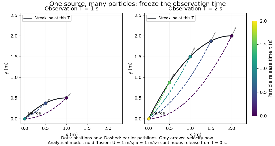
Each panel fixes one observation time. Coloured dots are the present positions of particles with the indicated release times; dashed pathlines show those particles' earlier histories. The black streakline connects present positions of the continuously released family, including release times between the sampled dots. After $T=1\mathrm{s}$, particles already present keep moving and new ones enter at the origin, so the later streakline is not a frozen record of the earlier one. Injection beginning only at $\tau =1\mathrm{s}$ would show just $0\le x\le 1\mathrm{m}$ of the $T=2\mathrm{s}$ curve. Both panels are diffusion-free analytical models, not experimental photographs.

Kline's contracting-channel demonstration switches from marking an element to continuous bubble production at a marking wire: the resulting trace is a streakline. The apparatus therefore changes the curve being displayed by changing the marking history, even with the same channel. A wire produces a family of traces; conceptually each fixed emitting location supplies its own streakline. Individual bubbles are markers rather than perfect fluid elements: Jean Hertzberg's teaching notes describe hydrogen production by electrolysis at a thin cathode wire and warn that larger bubbles have more buoyancy. ^{[ref] [ref]}

A dye version uses a small fixed injection port upstream in a transparent water channel, a dilute premix of dye with the channel water, illumination and a fixed optical camera. Start continuous injection at a recorded time ${\tau }_0$ and take a short exposure at $T$: the visible filament approximates a streakline, not the accumulated pathline of one particle. Repeat with the same port and imaging geometry after changing the flow with time; compare the filament against local directions estimated from short displacements of sparse markers at $T$. Agreement in a steady flow and possible disagreement when the flow changes are the predictions being tested; no measured curves are claimed here. The protocol follows Hertzberg's advice to use small ports, little injected volume and a dilute premix with matched density and viscosity. Check for nozzle disturbance by reducing injection rate, for buoyancy by watching the premix in still water, and for diffusion by comparing filament widths at different ages. Keep exposure short enough to suppress motion blur. Dye concentration approximates a passive scalar only when it has negligible feedback on the velocity field; finite port width, diffusion and out-of-plane motion limit how literally a visible filament can be read as a geometrical streakline. ^[ref]

For a point $B$ of a curve, let its ordinate meet the chosen coordinate axis at $C$, and its tangent meet that axis at $E$. The segment $CE$ is the subtangent. It depends on the chosen axis. For the standard parabola, $CE=2CD$, where $D$ is its vertex of a parabola.

A system of equations requires one choice of unknowns to satisfy several equations at once. Its solution set is the intersection of the solution sets of the individual equations. For example, $x^2+y^2=1$ and $y=(x-1{)}^2$ ask for intersections of a unit circle and a parabola. A linear system is the special case in which every equation is linear in the unknowns.

A tangent vector at a point $p$ of a smooth manifold without boundary records an instantaneous velocity through $p$. Its base point is part of the data; measuring its length additionally requires a Riemannian metric. Intrinsically, a smooth curve $\gamma$ with $\gamma (0)=p$ defines its tangent vector by how every local smooth function changes along it:This is a derivation at a point. Two smooth curves through $p$ represent the same tangent vector if these derivatives agree for every such smooth function; equivalently, their coordinate velocity vectors agree in one manifold chart. The chain rule makes that agreement independent of the chosen manifold chart. ^[ref]

For an embedded submanifold of Euclidean space, the intrinsic tangent vector is represented by the ordinary derivative ${\gamma }^{\prime }(0)$, with its base point $p$ retained. A drawn arrow starting at $p$ represents that tangent vector; its endpoint $p+{\gamma }^{\prime }(0)$ need not lie on the embedded submanifold. Nor is a tangent vector required to be a unit tangent vector: a stationary smooth curve gives the zero vector, which belongs to the tangent space but has no direction to normalize.

Here are explicit calculations. In ${\mathbb{R}}^2$, $\gamma (t)=(t,t^2)$ and $\eta (t)=(t,2t^2)$ have different routes but the same tangent vector $(1,0)$ at $(0,0)$. For $f(x,y)=3x+y$, both give $v(f)=3$. For a circle of radius $R$, $c(t)=(R\cos (\omega t),R\sin (\omega t))$ has tangent vector $(0,R\omega )$ at $(R,0)$: changing $\omega$ changes the speed or reverses travel without changing the circle.

A reparametrization $\beta (s)=\gamma (h(s))$ with $h(0)=0$ gives, by the chain rule, ${\beta }^{\prime }(0)=h^{\prime }(0){\gamma }^{\prime }(0)$. A regular change of curve parameter has $h^{\prime }(0)\ne 0$. The singular choice $h(s)=s^3$ instead givesBoth describe the same parabola, whose tangent line at the origin is still the horizontal axis. The zero velocity diagnoses this singular change of curve parameter, whose inverse is not differentiable at zero; it does not show that the geometric tangent line is absent. The regular curve $\gamma$ supplies its nonzero direction.

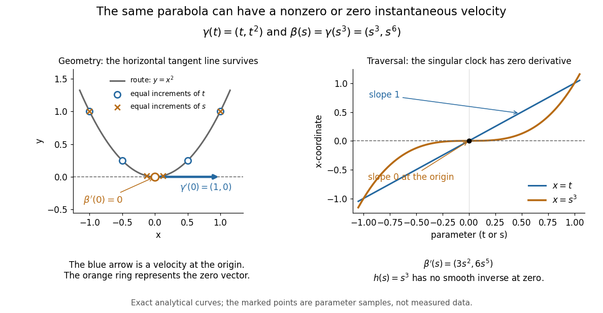
The diagram is an analytical illustration of these exact parametric curves, with equal parameter increments marked on each route. It separates geometry from traversal: the tangent line depends on the route, while a velocity vector also depends on how the curve parameter advances.

For a regular curve $\mathbf{r}(t)$ with nonzero velocity vector, its unit tangent vector isThe Euclidean norm in the denominator removes the traversal speed, leaving a unit vector that records direction. A positive change of traversal speed leaves this direction unchanged; reversing the direction of travel reverses $T$. In arc length coordinates, $T=d\mathbf{r}/ds$.

For the parabola $\mathbf{r}(t)=(t,t^2)$, the velocity vector is $(1,2t)$ and the speed is $\sqrt{1+4t^2}$. At $t=1$, $T=(1,2{)}^T/\sqrt{5}$. The tangent vector $(1,2{)}^T$ and the unit tangent vector point in the same direction, but only the latter has Euclidean norm one. The principal normal vector is a further choice based on how this direction changes, where the curvature is nonzero. ^[ref]

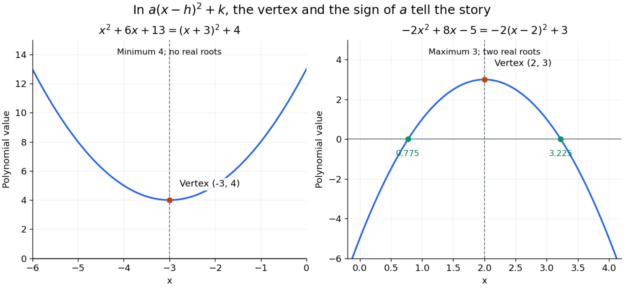
Write the quadratic polynomial asIts function graph is a parabola with vertex of a parabola $(h,k)$. Equal offsets from $h$ give equal values, since $p(h+t)=p(h-t)=a{t}^2+k$. If $a>0$, the minimum is $k$; if $a<0$, the maximum is $k$. In both cases it is attained only at $x=h$.

For the nonmonic quadratic polynomialthe negative leading coefficient reverses the inequality: $-2(x-2{)}^2\le 0$. Its maximum is $3$ at $x=2$. Its coefficients are different from those of the positive example, but the same form exposes the shape of both function graphs.

Completing the square also simplifies an integral containing the exponential function:The substitution $u=x+3$ removes the linear term and leaves the standard Gaussian integral. The same shift that locates the minimum makes this integral recognizable.

For a parabola described by the function graph $y=a(x-h{)}^2+k$, with nonzero $a$ in the real numbers, its vertex of a parabola is the point $(h,k)$. This point gives its minimum or maximum value of $y$ in these coordinates.