Past exam of the chemistry course of the year 3 of the natural sciences course of the University of Cambridge / 2022 / Paper 2B / Section B

For a self-adjoint Hamiltonian bounded below, every nonzero admissible trial wavefunction satisfies the quantum variational principleHere $E_0$ is the lowest exact energy, and the trial function must obey the physical boundary conditions and have finite relevant integrals. Equality holds for a wavefunction in the ground-state eigenspace. The quotient is unchanged by normalization or any nonzero overall scalar.

Expand the trial wavefunction in a complete orthonormal set of exact eigenfunctions, $\psi ={\sum }_n{c}_n{\varphi }_n$, with $\hat{H}{\varphi }_n=E_n{\varphi }_n$ and $E_n\ge E_0$. The coefficients may depend on any chosen variational parameters. Orthogonality removes the cross terms in both integrals, givingConsequentlyThis proves the quantum variational principle. The denominator is positive because the trial function is nonzero. Equality requires every occupied exact state to have $E_n=E_0$, allowing for ground-state degeneracy. With a continuous part of the spectrum, the corresponding nonnegative spectral integral gives the same conclusion.

Write $g=e^{-q^2/2}$ and $f=2q^2-a$. Product differentiation for the reduced quantum harmonic oscillator givesFor an eigenfunction, this must equal $E(2q^2-a)g$ at every $q$. Matching the $q^2$ coefficients gives $E=5/2$, and matching constants then gives $5a/2=2+a/2$. Hence $a=1$ and $E=5/2$. This is the even $n=2$ oscillator state. Its normalized wavefunction is ${\varphi }_2=(2q^2-1)e^{-q^2/2}/(\sqrt{2}{\pi }^{1/4})$.

Direct evaluation of the Rayleigh quotient exposes a problem with the requested minimization. Using the supplied Gaussian integrals,ThusThe eigenfunction value $a=1$ is a maximum, not a minimum. Indeed $\mathcal{E}(1)=5/2$, whereas $\mathcal{E}(0)=11/6$ is already lower. There is no finite minimizing $a$ in this family: its infimum is $1/2$, approached as $|a|\to \infty$, when the normalized trial wavefunction approaches the ground state. This is consistent with the quantum variational principle. The original printed instruction in this subpart is therefore inconsistent as an unconstrained minimization; a stationary Rayleigh quotient need not be a minimum.

The intended excited state can instead be obtained by imposing an excited-state variational constraint. Orthogonality to the ground state requireswhich fixes $a=1$. Every member of the family is even, so it is already orthogonal to the odd $n=1$ state. With the ground state excluded, the lowest allowed oscillator energy is therefore $E_2=5/2$. In the exact oscillator basis, $\psi$ is proportional to $\sqrt{2}{\varphi }_2+(1-a){\varphi }_0$, making both the maximum and the orthogonality correction transparent.

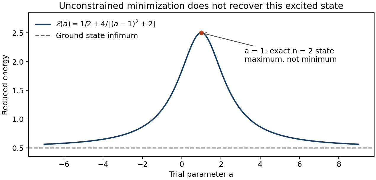
Exact solutions of the Schrödinger equation are unavailable for most interacting or realistic molecular systems. The quantum variational principle turns the search for a ground-state wavefunction into optimization of a computable energy quotient in a tractable trial family. The result is an upper bound: enlarging a nested trial space can only lower or preserve the optimized energy, providing a systematic convergence check. Trial functions can incorporate boundary conditions and known symmetry before calculation. Near an exact normalized ground state, a small orthogonal wavefunction error changes the energy only to second order, which explains why useful energies can result from imperfect trial functions. This does not ensure that every other observable is equally accurate, nor that a restricted trial family captures correlation adequately. Excited states require orthogonality or appropriate symmetry restrictions; unrestricted minimization seeks the ground state, as the preceding calculation demonstrates.

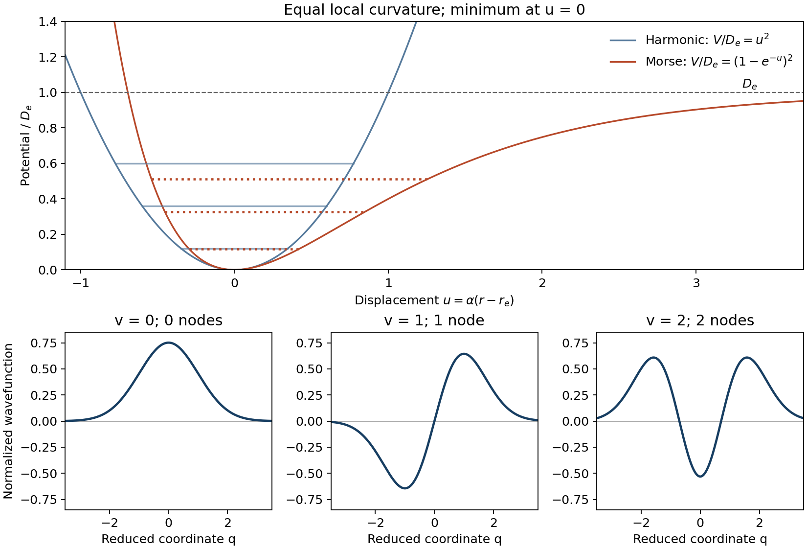
Let $u=r-r_e$ measure displacement from the equilibrium bond length and put the minimum of potential energy at zero. The harmonic model and the Morse potential areThe harmonic approximation is a symmetric parabola and has no dissociation limit. The Morse potential has a steep compressed side and a shallower extended side, approaching $D_e$ as $r\to \infty$. Matching the curvatures at the minimum gives $k=2D_e{\alpha }^2$. With $\tilde{\omega }$ denoting a spectroscopic wavenumber rather than an angular frequency, the energy levels areHere $x_e$ is the dimensionless spectroscopic anharmonicity constant. The harmonic spacing is constant, while the Morse oscillator spacing is $E_{v+1}-E_v=hc\tilde{\omega }[1-2x_e(v+1)]$ and decreases as the levels approach dissociation. Only finitely many Morse oscillator levels are bound. The exactly solvable potential was introduced to model this anharmonic behaviour.^[ref]

For the harmonic model put $q=\sqrt{\mu \omega /\hslash }u$, with $\omega =2\pi c\tilde{\omega }$, and $N={\pi }^{-1/4}$. The first three normalized reduced-coordinate wavefunctions areTheir numbers of nodes are zero, one and two, and their parities are even, odd and even. The $v=2$ nodes are at $q=\pm 1/\sqrt{2}$. The diagrams below use analytic curves and arbitrary illustrative scales, with both potentials given the same local curvature.

Write $s=v+1/2$ and complete the square in the Morse oscillator energy:The finite bound-level sequence approaches the dissociation limit at the vertex of this extrapolated parabola. Thus the bond potential-well depth isThe continuous vertex is a convenient way to identify the limit; it is not an additional normalizable bound level at the threshold.

The ground-state dissociation energy starts at the lowest vibrational level, rather than the minimum of the potential. The zero-point energy of the Morse oscillator isSubtracting it from the bond potential-well depth givesThis distinction matters whenever a dissociation energy is inferred from a vibrational spectrum.

The strong band is the $v=0\to 1$ vibrational fundamental, and the weaker band near twice its wavenumber is the $v=0\to 2$ first vibrational overtone. At room temperature these high-frequency oscillators have overwhelmingly ground-state vibrational populations. In the harmonic-potential, linear-dipole limit the infrared selection rule is $\Delta v=\pm 1$; anharmonicity and nonlinear dipole dependence make the overtone weakly allowed. A $1\to 2$ hot band would lie near, and slightly below, the fundamental wavenumber, rather than near twice it.

Let $f$ and $o$ denote the measured fundamental and first-overtone wavenumbers, and put $y=\tilde{\omega }{x}_e$. Differences of the Morse oscillator levels giveConsequently $x_e=y/\tilde{\omega }$, $D_e/(hc)={\tilde{\omega }}^2/(4y)$ and $D_0/(hc)=D_e/(hc)-(\tilde{\omega }/2-y/4)$. Substituting the two pairs of measured bands gives the following derived quantities:The conversion is $1\mathrm{c}{\mathrm{m}}^{-1}=0.0119626566\mathrm{kJ}\mathrm{mo}{\mathrm{l}}^{-1}$, after multiplication by $N_{A}hc$ and consistent length units. Therefore the requested ground-state dissociation energies are $D_0(\mathrm{A})=448.4\mathrm{kJ}\mathrm{mo}{\mathrm{l}}^{-1}$ and $D_0(\mathrm{B})=388.5\mathrm{kJ}\mathrm{mo}{\mathrm{l}}^{-1}$. The corresponding potential-well depths are $D_e(\mathrm{A})=464.1$ and $D_e(\mathrm{B})=402.2\mathrm{kJ}\mathrm{mo}{\mathrm{l}}^{-1}$. These are extrapolations under the stipulated Morse oscillator model; two low-lying bands do not establish the accuracy of the real potential near dissociation.

The molecule with the larger inferred dissociation energy is assigned the stronger hydrogen–halogen bond: $\mathrm{A}=\mathrm{HBr}$ and $\mathrm{B}=\mathrm{HI}$. Moving from bromine to the larger iodine atom generally lengthens the bond and reduces effective overlap with the compact hydrogen $1s$ orbital, so hydrogen iodide is more weakly bound. Independently, the tabulated ground-state harmonic constants near $2649\mathrm{c}{\mathrm{m}}^{-1}$ for hydrogen bromide and $2309\mathrm{c}{\mathrm{m}}^{-1}$ for hydrogen iodide agree with the inferred assignment.^[ref][ref] The ordering is the identification criterion; the low-level Morse oscillator extrapolations above should not be presented as measured dissociation energies.

The operator ${\hat{J}}_z$ describes the $z$ component of angular momentum, whereas ${\hat{J}}^2$ describes its total squared magnitude. For a spherical harmonic $Y_{JM}$ the corresponding eigenvalues areThus the magnitude is $\hslash \sqrt{J(J+1)}$, not $J\hslash$. For ordinary orbital rotation $J=0,1,2,\dots$ and $M=-J,-J+1,\dots ,J$. The simultaneous values are possible because these two operators commute.

Normalization of a wavefunction on the unit sphere uses solid angle $d\Omega =\sin \theta d\theta d\varphi$, not the flat measure $d\theta d\varphi$. Since $|e^{-i\varphi }|=1$,where $u=\cos \theta$. ThereforeWith the usual phase convention this is the spherical harmonic $Y_{1,-1}$. An arbitrary global unit-modulus factor would not change normalization or any observable.

The azimuthal derivative is ${\partial }_{\varphi }\psi =-i\psi$, so ${\hat{J}}_z\psi =(-i\hslash )(-i)\psi =-\hslash \psi$. For the polar part of the angular Laplacian,Their sum is $-2\sin \theta e^{-i\varphi }=-2\psi$, hence ${\hat{J}}^2\psi =2{\hslash }^2\psi$. Comparing these two eigenvalues with $M\hslash$ and $J(J+1){\hslash }^2$ gives $J=1$, $M=-1$. The sign of $M$ follows from both minus signs in the ${\hat{J}}_z$ calculation.

For a linear rigid rotor, dividing the angular momentum squared eigenvalue by twice the moment of inertia givesThe quantum degeneracy counts the values $M=-J,\dots ,J$ with the same energy. It excludes nuclear-spin multiplicity and any fine or hyperfine splitting absent from this model.

Express the rotational constant as a spectroscopic wavenumber $\tilde{B}=h/(8{\pi }^{2}cI)$. The rotational absorption selection rule $\Delta J=+1$ givesSuccessive lines therefore have spacing $2\tilde{B}$, regardless of the starting $J$. Both observed spacings are $20.88\mathrm{c}{\mathrm{m}}^{-1}$, giving $\tilde{B}=10.44\mathrm{c}{\mathrm{m}}^{-1}$. The three lines are consequently the $5\to 6$, $6\to 7$ and $7\to 8$ transitions within the stated precision; the first observed line is not the $0\to 1$ line.

Using the given isotopic masses, the reduced mass isWith $\tilde{B}=1044{\mathrm{m}}^{-1}$ and $c$ in $\mathrm{m}{\mathrm{s}}^{-1}$, the bond length follows fromThe small common $0.01\mathrm{c}{\mathrm{m}}^{-1}$ offset relative to integer multiples of the spacing is immaterial at the precision of this model. A real ground-vibrational-state rotational constant determines an effective vibrationally averaged bond length; it need not equal the exact equilibrium separation.

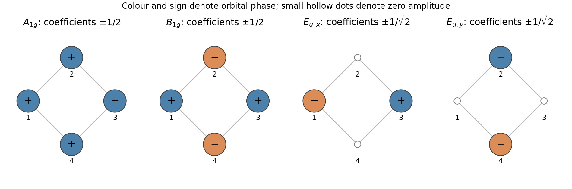
The drawn $x,y$ axes pass through opposite sites, rather than along the square edges. In the D4h molecular point group class order $(E,2C_4,C_2,2C_2^{\prime },2C_2^{\prime \prime },i,2S_4,{\sigma }_h,2{\sigma }_v,2{\sigma }_d)$, an s orbital contributes $+1$ whenever its centre is fixed and zero otherwise. ThusFor example, a transverse twofold rotation about the printed $x$ axis fixes sites 1 and 3, while its diagonal counterpart exchanges all four sites. Reflection in the square plane fixes every site. Taking character inner products, with class sizes $(1,2,1,2,2,1,2,1,2,2)$, givesThese have dimensions $1+1+2=4$. The $B_{1g}$ label is tied to the printed diagonal-axis convention; rotating the transverse coordinate labels by $45^{\circ }$ would interchange $B_{1g}$ and $B_{2g}$.

Treat the site atomic orbitals $s_1,\dots ,s_4$ as orthonormal, as in the Hückel method. A normalized set of symmetry-adapted linear combinations isThe first combination is unchanged by every operation; the alternating combination has the transformation signs of $x^2-y^2$ for the printed axes. The last two transform together like $(x,y)$. The squared coefficients sum to one in each case, and their pairwise inner products vanish. Any orthogonal rotation of the two $E_u$ combinations is an equally valid basis for that degenerate subspace.

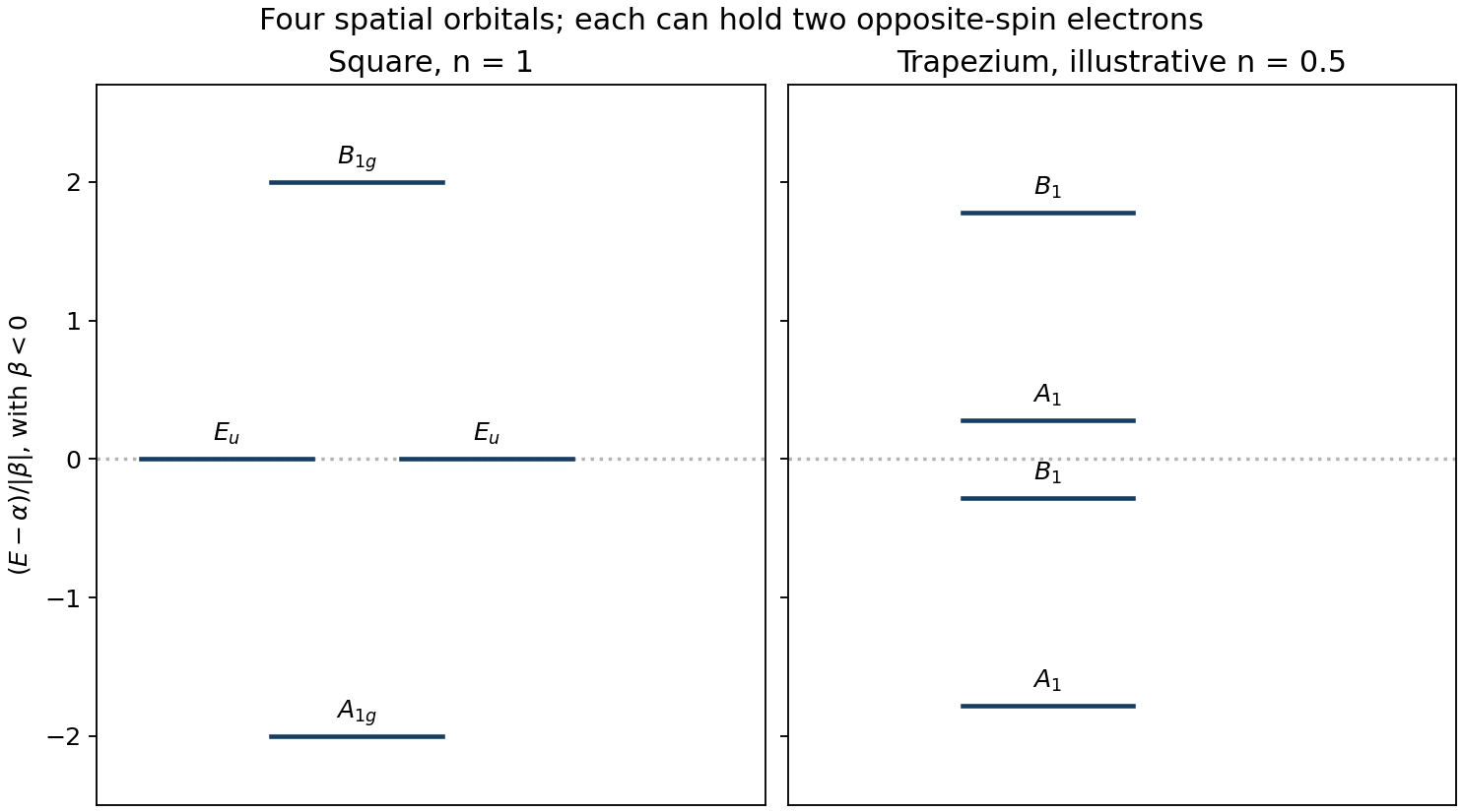
Use a common Coulomb integral $\alpha$ on each site, a resonance integral $\beta$ on each adjacent pair, zero interaction across a diagonal, and the identity overlap matrix. In site order $(1,2,3,4)$ the Hückel method givesApplying it to the four symmetry-adapted linear combinations givesFor the conventional bonding sign $\beta <0$, the all-in-phase combination is lowest and the alternating combination is highest. The $E_u$ combinations have canceling nearest-neighbour interactions and are nonbonding within this model.

The molecular orbital diagram has one level at $\alpha +2\beta$ labelled $A_{1g}$, two degenerate levels at $\alpha$ labelled $E_u$, and one level at $\alpha -2\beta$ labelled $B_{1g}$, in increasing energy for $\beta <0$. Each spatial molecular orbital admits two opposite-spin electrons. The diagram below also shows how one representative distortion lifts the middle degeneracy; the distorted scale is illustrative, not a fitted molecular spectrum.

Use the trapezium's printed axes, with principal axis $z$ in its plane and $y$ perpendicular to the plane. For either site pair $(1,2)$ or $(3,4)$, the group representation has characters of a representation $(2,0,2,0)$ in the order $(E,C_2(z),\sigma (xz),\sigma (yz))$: identity and the molecular-plane mirror fix both s orbitals, while the other two operations exchange them. The character inner products give ${\Gamma }_{12}={\Gamma }_{34}=A_1\oplus B_1$ in the C2v molecular point group.

Within each pair the in-phase and out-of-phase combinations have $A_1$ and $B_1$ symmetry respectively. One normalized choice isThe sign convention for $d$ is chosen to make the off-diagonal interaction positive in the corresponding two-by-two block. It does not change the physical predictions. These are pair symmetry-adapted linear combinations; the actual molecular orbitals are linear combinations within each of the two equal-symmetry pairs, found by diagonalizing the blocks.

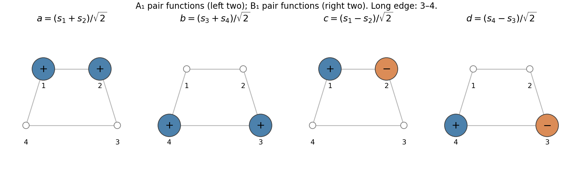
The long edge is $3$–$4$. In the orthonormal pair basis $(a,b)$, its weaker resonance integral $n\beta$ changes the second diagonal element. The two short side edges contribute an inter-pair matrix element $\beta$, givingWith $\lambda =(E-\alpha )/\beta$, its secular equation isThe eigenvalues are thereforeAt $n=1$ they become $\alpha +2\beta$ and $\alpha$, agreeing with the square limit. Symmetry permits mixing of the two $A_1$ pair functions; treating each pair as an isolated bond would miss the off-diagonal term.

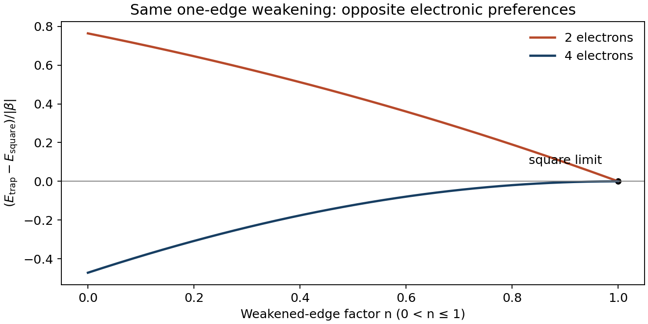
Put $D=\sqrt{n^2-2n+5}=\sqrt{(n-1{)}^2+4}$. For $0<n<1$, $D>n+1$, since $D^2-(n+1{)}^2=4(1-n)>0$. Remembering $\beta <0$, the two lowest trapezium molecular orbital energies areThe remaining levels lie at $2\alpha -{ϵ}_2$ and $2\alpha -{ϵ}_1$. Filling the lowest spatial orbitals with opposite-spin pairs givesFor the square four-electron case, two electrons occupy the lowest orbital and two occupy the degenerate $E_u$ set. Their summed one-electron energy is fixed here, but this Hückel method calculation alone does not decide the spin or correlation within that open shell.

For two electrons, $n+1+D<4$ whenever $0<n<1$: both sides of $D<3-n$ are positive and squaring reduces the inequality to $n<1$. Since $\beta <0$, the trapezium then has a higher total electronic energy than the square. The two-electron model favours the square. For four electrons, $D>2$, so $2\beta D<4\beta$: the four-electron model favours the distortion toward a trapezium. The lower split middle orbital is occupied while the upper one is empty.

The distinction is especially clear near the square. Write $\delta =1-n>0$; then $D=2+{\delta }^2/4+O({\delta }^4)$ andIn particular the four-electron lowering in this specified one-edge model is quadratic near the square; a first-order lowering of the entire occupied sum should not be asserted merely from the middle-level splitting. This Hückel square-to-trapezium distortion is an electronic comparison under the stated fixed-$\alpha$, fixed-short-edge-$\beta$ assumptions. Nuclear repulsion, other bonding contributions and the structural cost of distortion are omitted, so an actual equilibrium geometry or optimum $n$ is not determined by this calculation alone.