Let and be two finite bases of the vector space . We prove the underlying exchange argument rather than assuming that dimension is already well-defined.
More generally, suppose are linearly independent and form a spanning set. Starting with the spanning list of 's, replace one of its members by . Indeed, express as a linear combination of that list; at least one coefficient is nonzero, so we can solve for its corresponding and retain a spanning list. Inductively, suppose the spanning list now consists of and of the original 's. Express in that list. Some coefficient of a remaining must be nonzero, since otherwise would lie in the span of the preceding 's, contradicting linear independence. Solve for that and replace it by .
If , after replacements the spanning list consists of , forcing to lie in their span, again a contradiction. Thus every finite linearly independent list has at most as many members as every finite spanning set. This proves the Steinitz exchange lemma in the form required here. Applying it to the two bases in both orders gives and , hence . The zero vector space has only the empty basis, which also fits the argument.
First quotient by , obtaining the quotient ringPolynomial division by this monic quadratic gives a unique representative with . Uniqueness holds because a nonzero multiple of a monic quadratic cannot have degree less than two. Therefore .
In characteristic three, . The residue is nonzero by the uniqueness of the degree-one representative, but . Thus is both a nilpotent element and a zero divisor. Consequently is not an integral domain. Equivalently, its multiplication is that of , rather than that of a field with nine elements.
We first justify the maximum in the proposed supremum norm. If a null sequence is nonzero, choose an index with . All sufficiently late terms have absolute value smaller than , since . Hence the largest absolute value occurs among a finite initial set of terms, and is finite. For the zero sequence the maximum is zero.
The norm axioms now follow directly. The maximum is nonnegative and vanishes precisely when every coordinate vanishes. For a scalar , . For two null sequences, coordinatewise addition remains a null sequence andTaking the maximum proves the triangle inequality, so this really is a norm on .
Let have a single in position . If , then . A convergent sequence in a normed vector space must be a Cauchy sequence, by the triangle inequality. These distances violate the Cauchy condition with, for example, . Thus does not converge in this norm, even though each fixed coordinate converges to zero.
The identity theorem can be expressed as the principle of isolated zeros: a holomorphic function on a connected open set is either identically zero or has isolated zeros. Locally this follows from its Taylor series: at a zero of a function which is not locally zero, factor the first nonzero power, with . Connectedness then rules out a nonempty open region of zeros unless the whole function vanishes.
Set . This is holomorphic on the punctured plane: reflecting and conjugating a local power series produces another power series. The absence of an essential singularity means that the singularity at zero is removable or a pole. Thus for some integer , extends holomorphically across zero; the same is true of . Their differencetherefore extends to a holomorphic function on all of . At every , real-valuedness gives . These zeros accumulate at zero, which is now an interior point of the domain of . The identity theorem forces . For we may divide by , yieldingThe conjugation outside is essential. Also, applying the identity theorem directly on the punctured plane would be invalid: the accumulation point zero does not belong to that domain.
Write . Separation of the axisymmetric Laplace equation in spherical coordinates, with regularity at the poles, gives the Legendre polynomial expansionThe discarded interior terms are singular at the origin; the discarded exterior terms fail the prescribed decay at infinity. Continuity at gives .
Take the radial derivative jump to mean the exterior derivative minus the interior derivative. ThenSince , comparison with the prescribed jump gives , , and all other coefficients zero. ThusThese expressions satisfy the Laplace equation, continuity, regularity and decay, and their jump is . If the opposite convention for the word jump is chosen, both expressions change sign. Although only the axisymmetric expansion is needed, no additional nonaxisymmetric solution can be added: zero jump and continuity glue such an addition into an everywhere regular harmonic function decaying at infinity, which vanishes by the maximum principle for harmonic functions.
For a normalized wavefunction, the probability density and probability current areThe Schrödinger equation and its conjugate, for a real potential, areMultiplying respectively by and and adding their expressions for the time derivatives cancels the potential terms. HenceThe gradient cross-terms cancel when expanding the divergence. ThereforeThis continuity equation expresses local conservation of probability. Integrating over a region says that its probability decreases by the outward flux of the probability current.
For a normalized wavefunction in the required operator domains and a self-adjoint operator , its expectation value and standard deviation areEquivalently the squared uncertainty is , which is visibly nonnegative. Since the expectation value of a self-adjoint operator is real, expansion of the square and giveFor a state not normalized to one, divide each defining expectation integral by before using this formula.
Orient the moving boundary consistently with the normal on a spanning surface . The relevant Maxwell equations are and .
First hold the magnetic field fixed at time and compare the fluxes through the old and new surfaces. The closed surface consists of the new surface, the reversed old surface, and the joining ribbon. A parametrization of the ribbon by boundary arclength and time gives its outward oriented area vector as . Thus its flux isBy the divergence theorem, the total flux through the closed surface is zero. Adding the field's explicit change in time consequently gives the moving-surface flux derivativeNow apply Stokes theorem and :Consequently the electromotive force, including the motional electromotive force, satisfiesThis derives the moving-circuit form of Faraday's law, including both changing fields and changing circuit geometry.
The successive divided differences for nodes areThus the Newton interpolation polynomial isExpanding the products gives the power formThe four values verify the data. Uniqueness follows because the difference of two degree-at-most-three interpolants would have four distinct roots.
Keep the original four-node interpolation polynomial . The correction must vanish at all four original nodes, so a degree-at-most-four interpolant has the formSince and the product at is , matching the new value gives , hence . Expanding yieldsIt takes the values at the five nodes. The same root-count argument proves uniqueness of this interpolation polynomial.
Let . The residue contains all information needed for the next residue, so is a four-state Markov chain. In the order , its transition matrix isFor example, from residue , a head returns to and a tail goes to ; from either odd residue the tail leaves that residue unchanged.
The stationary distribution solves . Its equations give , , and . Normalization therefore givesThe Markov chain is irreducible: the positive-probability transitions around reach all states. It is also aperiodic because it has self-loops. The finite irreducible Markov chain ergodic theorem says that empirical state frequencies converge almost surely to the unique stationary distribution, irrespective of the initial state. HenceAperiodicity also permits convergence of the one-time state probabilities, although it is not needed for this empirical-frequency theorem.
An orthogonal transformation preserves the real inner product. If is an invariant subspace, its orthogonal complement is invariant too: in finite dimensions, and for , , we have .
Complexify the space and the transformation. There is a complex eigenvalue , and preservation of the Hermitian norm gives . If is real, it is or , and the real kernel of contains a nonzero vector. Its span is an invariant line on which acts as or .
If is nonreal, write an eigenvector as . Its real and imaginary parts are linearly independent: otherwise a nonzero real vector would have the nonreal eigenvalue. The real plane is invariant, because comparison of real and imaginary parts in gives real combinations of . The restriction has determinant . In an oriented orthonormal basis of , it is therefore a rotationThere is no invariant real line in this plane: such a line would supply a real eigenvalue, whereas its two eigenvalues are nonreal.
Apply the argument repeatedly to the invariant orthogonal complement. Thus the smallest mutually orthogonal invariant blocks are lines with action , and planes with a genuine rotation. Planes with angle or can be decomposed further into lines.
In dimension three a suitably chosen orthonormal basis therefore gives eitherorChanging the orientation of the plane reverses the angle, so this angle range loses no cases. These exhaust rotations, reflections and their possible compositions in three dimensions.
Let be the commutative subring of endomorphisms generated by scalar multiplication and . Commutativity follows because the scalar maps commute with the -linear map , and every element of is a polynomial in with scalar coefficients. Thus determinants and the adjugate identity apply to matrices over .
With the convention for the coefficients in the question, the column of generators satisfiesMultiply by over . Since , the endomorphism kills every generator . It therefore kills every element of the module, by -linearity. Hence it is the zero endomorphism, andThe argument does not require the generating set to be a basis; relations among the generators cause no difficulty. This is the determinant trick.
A finite basis is a generating set, so the preceding determinant trick applies with and . If , the map sending to is a ring homomorphism. Since a determinant is a polynomial expression in its entries, it sends to . ThusWith the more usual monic characteristic polynomial , this reads , the Cayley-Hamilton theorem. If the matrix convention uses column coordinates instead of the row convention above, transpose ; its characteristic polynomial is unchanged.
In the Poincare disc model, hyperbolic lines are diameters and circular arcs meeting the boundary circle orthogonally. In the upper half-plane model, they are vertical lines and semicircles with centres on the real axis. The metric is conformal, so hyperbolic perpendicularity agrees with Euclidean perpendicularity.
Use an isometry of the hyperbolic plane to send an arbitrary line to the positive imaginary axis. For with , a point on that axis is with . The hyperbolic distance formula givesPut . The last expression is , uniquely minimized at , since with equality only there. Hence the unique closest point is . The semicircle passes through and and meets the imaginary axis at a right angle. Conversely a semicircle centred at a real number can meet that axis orthogonally only if ; a vertical line cannot furnish such a crossing. Thus the perpendicular is unique. Isometries transfer both uniqueness and minimization back to the original line.
For on the specified second semicircle, and . Its perpendicular to the axis is the semicircle just found, with radius . MoreoverSince for , we obtainThis is uniform over the whole semicircle, including points arbitrarily close to the ideal endpoints.
Finally send any first line of an ultraparallel pair to the axis by an isometry of the hyperbolic plane. The second cannot be a vertical line, since that would share the ideal point at infinity. Its two finite endpoints lie on the same side of zero; otherwise its semicircle would meet the axis, or share the endpoint zero. Reflect horizontally if necessary, so those endpoints are with . The uniform estimate above then givesThus ultraparallel hyperbolic lines have strictly positive separation; disjointness in the interior alone would not suffice.
The contraction mapping theorem says that if a nonempty complete metric space has a map satisfying for every and some fixed , then has a unique fixed point , and for every starting point. In particular ; an estimate using only consecutive iterates is .
Let and for . Direct subtraction givesThus every iterate after the first lies in . On this interval,The mean value theorem gives a uniform Lipschitz constant , and maps the interval into itself. The interval is closed in , hence complete. By the contraction mapping theorem, its iterates converge to its unique fixed point, which is . Therefore every positive initial guess converges to .
The local error satisfies the sharper exact recursionIn relative error , this is . Thus when , the next relative error is approximately : one step roughly doubles the number of correct decimal digits. In particular one further step suffices for one additional digit once the iteration is sufficiently close. For absolute-error accuracy, the precise sufficient condition gives ; this states explicitly how close is sufficient when has an arbitrary scale.
Let be a compact subset of a Hausdorff space, and take . For each , the definition of a Hausdorff space supplies disjoint open neighbourhoods of and of . Compactness gives finitely many covering . Their corresponding intersection is open, contains , and misses . Therefore every point of the complement has an open neighbourhood contained in the complement, so is closed. The empty compact set is closed as well.
The nearest-point assertion requires . If , there is no possible point , so the literal assertion for every closed subset has that exception.
For a nonempty closed subset of a compact metric space, is itself compact. The function is continuous, since by the triangle inequality. The extreme value theorem therefore gives a minimizer , with
Now assume the midpoint property and suppose were disconnected. There would be nonempty disjoint relatively open sets with . Each is also closed, hence compact. The continuous distance function on the compact product attains its minimum . It is positive, since a zero value would imply .
Choose a midpoint of this minimizing pair. It lies in either or . In the first case contradicts minimality; in the second, does. Thus the midpoint property forces to be connected. The empty space is connected by the usual no-separation definition, so it also causes no exception here.
For example, it suffices to assume . Indeed the absolute double integral isThus Fubini's theorem permits interchange in the Fourier transform of the convolution. With ,Hence the convolution theorem in this normalization isThere is no extra in this formula; that factor belongs to the inverse transform and Parseval identity for the convention being used.
Integrating the interval indicator givesThe convolution is the length of overlap of two intervals of length one whose centres differ by . Thus for , and zero otherwise. The convolution theorem givesFor this Fourier transform normalization, the Parseval identity says . Sincewe have . Substituting givesThe quotient at zero is understood by its continuous limit.
For a variation with but arbitrary , differentiation and integration by parts giveFirst choose variations supported inside the interval. The fundamental lemma of the calculus of variations gives the Euler-Lagrange equation. Then allow arbitrary endpoint variation to obtain the natural boundary conditions for a free endpoint:Because has no explicit dependence on ,Thus the Beltrami identity is , constant along an extremal.
For the brachistochrone problem, put , so conservation of energy gives the bead speed . Its travel time isThe Beltrami identity now gives for a positive constant . A descending cycloid parametrizes this relation:The free endpoint has , hence . On the first descending arc this occurs at . ThereforeAlong this arc and , soThe initial vertical tangent causes no divergent travel time: the quotient has the finite constant limit .
To verify global minimality, take any admissible wire graph of finite travel time below the release level, and let be its maximum depth. For , the Cauchy-Schwarz inequality givesIndeed the two coefficients on the right, after multiplication by , form a unit vector. Since the path starts at depth zero and reaches depth , the weighted total variation is at least the integral over all depths from to . ConsequentlyThe last inequality is minimized at . Our cycloid attains equality throughout: its depth increases to and . Thus it achieves the genuine minimum over the wire graphs, not merely a stationary time. Reflection handles a negative horizontal endpoint coordinate by replacing with .
The Lorentz factor for isThe javelin's length at simultaneous barn-frame times follows from length contraction:Its proper length remains four metres.
In the javelin's rest frame, the barn moves at speed . Applying length contraction to its proper length givesThe lengths in the two frames use different pairs of simultaneous endpoint events.
Choose the barn entrance as , its exit as , and the positive direction as the javelin's motion. Put at the trailing end entering the barn. Write and in metres. In the javelin frame let the trailing end have , the leading end , and use the same origin event. The Lorentz transformation isIn the barn frame, the four world lines areIn the javelin frame they areThe two spacetime diagrams below use vertical time coordinates and horizontal spatial coordinates. Event labels refer to the same physical events in both panels; dashed lines show light-ray directions.
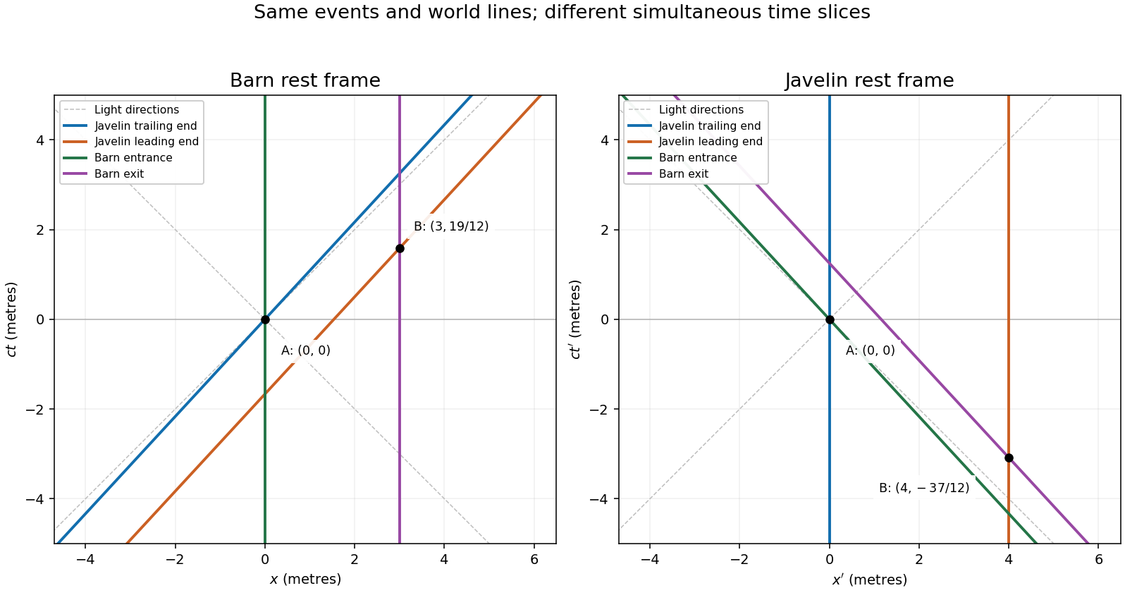
Javelin and barn world lines in the barn and javelin rest frames, with entry event A and exit event B
. Details. 
Event is the chosen origin. At , the leading-end world line reaches , soThe Lorentz transformation givesFor example . The squared spatial separation minus squared time separation isequally in the other frame. Thus and have spacelike separation.
In the barn frame, for the trailing end has entered while the leading end has not yet exited, so the whole javelin is inside at each simultaneous time slice. In the javelin frame the barn is shorter than the javelin and there is no simultaneous slice on which it contains the whole javelin. Also precedes there. This is consistent because relativity of simultaneity changes which endpoint events are simultaneous; the ordering of events with spacelike separation is not invariant. The physical intersections of the four world lines are the same in both diagrams.
Take the undisturbed free surface as , the bottom as , and the walls as . For an incompressible flow which is an irrotational flow, write with a velocity potential satisfying . Impermeability gives at the bottom, at the walls, and at the walls.
For the actual surface , the exact kinematic boundary condition for a free-surface graph isThe Unsteady Bernoulli equation, with atmospheric pressure at the surface and its time-dependent constant absorbed into , givesFor small disturbances about fluid at rest, and are first order. Products of first-order quantities and Taylor corrections from evaluating at are second order. The linear surface conditions are thereforeor, after eliminating the elevation,
The separated normal modes of surface gravity waves in a rectangular tank havewhere are nonnegative integers not both zero. The horizontal factors satisfy the wall conditions, and the vertical factor satisfies both the Laplace equation and the bottom condition. At the top, ; substitution into the surface condition givesThe elevation isReal physical standing waves are the real parts or linear combinations of these complex modes. The uniform mode has zero frequency and would change the mean depth; conservation of the fixed water volume excludes it from the disturbances. Modes with equal are degenerate and can be superposed.
Write the common variance as . Independence and the normal distribution giveMoreover and are independent. To see both assertions, standardize the observations into an isotropic Gaussian vector and choose an orthonormal basis with first vector . Its first coordinate is ; the remaining independent standard normal coordinates have squared sum . The same argument applies to the sample, independently of the first sample.
Under the null hypothesis, the difference of sample means is . The residual sums of squares add to an independent chi-squared distribution with degrees of freedom. Define the pooled sample variance and test statistic byFor , under this is with independent and . Hence under the null, the Student t-distribution.
Let be its 99th percentile. For the specified one-sided alternative, reject precisely whenBecause this distribution is continuous, the rejection probability under is exactly , irrespective of the nuisance mean and variance. Large positive values supply evidence for ; a two-sided or 0.995 cutoff would test a different alternative. The common-variance and independence assumptions are essential to this exact Student t-test. If both samples have size one, there are no residual degrees of freedom and the proposed unknown-variance test cannot be formed.
Use two-phase simplex to handle the constraint of the opposite inequality direction. Introduce nonnegative slack variables , a surplus variable , and an artificial variable . The equality constraints areFor Phase I maximize , initially with basis . Its initial simplex dictionary isChoose to enter. The simplex ratio test compares , and , so leaves. The new dictionary isSince , choose to enter. Its limiting ratios are from and from , so leaves. This givesNow , so let enter. Its limiting ratios are from and from ; the artificial variable leaves. The simplex dictionary becomesSetting all nonbasic variables to zero gives , a feasible original basis. Since , Phase I is optimal with value zero; delete .
For Phase II the original objective in this basis isAll nonbasic reduced costs are strictly negative, so no further improving simplex pivot exists. As the nonbasic variables are nonnegative, the dictionary also directly certifies , with equality only when . ThereforeThe second original constraint has slack five and the other two are tight. As an independent linear programming optimality certificate, multiply the first constraint by and the third, after reversing it, by . This gives , and subtracting proves the same upper bound for the objective.
Articles by others on the same topic
There are currently no matching articles.