The empirical distribution function gives each observation mass :The Glivenko-Cantelli theorem asserts the uniform, almost sure convergenceNo continuity of the distribution function is required. Here is a proof that also handles its jumps. Let be independent uniform random variables on , and write , where . The generalized inverse property gives , so, if is the empirical distribution function of the , then .
For a fixed positive integer , the strong law of large numbers applied at each of the finitely many grid points shows that almost surely. If , monotonicity sandwiches between its endpoint values, whenceTake the probability-one intersection of these events over all . On that event the limit superior is at most for every , hence is zero. Therefore . The coupled sequence has the same joint law as any independent sample from , which proves the asserted almost sure conclusion for the original sample.
For , the sample quantile iswhere denotes the th order statistic, with repeated observations retained. Suppose the population median is unique and is continuously differentiable in a neighbourhood of , with probability density function . ThenTo see the variance directly, fix and count observations below . This count has a binomial distribution with success probability . The event that the sample median is below this point is that the count is at least . The central limit theorem for this binomial triangular array gives a limiting probability , exactly the displayed normal distribution. Centering is necessary for stating the limiting distribution; subtracting the deterministic population median has no effect on the asymptotic variance requested in the comparisons.
For the standard normal distribution, and , so the sample median has asymptotic variance under scaling by . The central limit theorem gives for the sample mean. Thus the sample median has times the asymptotic variance of the sample mean, and its asymptotic relative efficiency against the sample mean is
This is a symmetric beta distribution with parameters , so its mean and median are both . At the median its probability density function is , giving asymptotic variance for the sample median. Direct integration givesConsequently . The sample median has times the asymptotic variance of the sample mean, with asymptotic relative efficiency
Write and for the individual and total score functions. Under the usual regularity assumptions, and , the nonsingular per-observation Fisher information matrix. The central limit theorem and weak law of large numbers giveRearranging the stipulated score expansion, including its remainder, givesSlutsky theorem therefore proves the asymptotic normality of a maximum likelihood estimator:A consistent plug-in Fisher information matrix yields the Wald statistic . Under the null hypothesis, , so a test of asymptotic size rejects when exceeds the quantile of that chi-squared distribution. A consistent observed Fisher information matrix gives the same limiting test.
With an -dimensional parameter of interest and nuisance parameter , partition accordingly. The marginal asymptotic covariance matrix of is the block of , whose inverse is the efficient informationThus the nuisance-adjusted Wald statistic is , with limiting null distribution . Using alone is generally incorrect when the nuisance parameter is estimated; it is valid when the cross-information vanishes.
For the Inverse Gaussian distribution in this problem, expand the exponent to obtain the log likelihood, up to terms independent of both parameters,Its score functions areFor each positive , the first score changes sign from positive to negative at , so this is the global maximizing mean parameter of an exponential family. Substituting it in the second score givesThe reciprocal function is strictly convex, so the denominator is positive for a nonconstant sample. The profile log likelihood is strictly concave in and tends to minus infinity at both endpoints, proving this is a maximum. Under continuous model sampling, a sample of size at least two is nonconstant almost surely. For a constant sample, including a one-observation sample, no finite joint maximum-likelihood estimator exists: the likelihood increases without bound as at .
For one observation, differentiating again and using givesThis parameter orthogonality proves that estimating does not reduce the efficient information for . The Wald statistic has the same algebraic form in the two cases:Using information evaluated at instead is another first-order equivalent convention.
The printed claim of coincidence needs a first-order interpretation. Known and unknown need not give numerically identical Wald statistics, because their maximum-likelihood estimators differ. With known, direct maximization givesFor example, observations and known give and . At , the displayed Wald convention gives and , respectively. Thus exact equality is false. Under the null hypothesis, however, , hence . Their centered, standardized estimates differ by , so their Wald statistics differ by . This is the valid asymptotic coincidence supplied by inverse Gaussian shape estimation and nuisance orthogonality.
For a nondegenerate distribution function , membership in its maximum domain of attraction means that there exist such thatat every continuity point of . A max-stable distribution satisfies: for each positive integer , there exist such that . Thus a maximum of independent copies has the same probability distribution after a change of location and scale.
Suppose first that . For fixed , the distribution functions have the two nondegenerate limitsThe given convergence-of-types result supplies constants such that . Equality extends from continuity points to all points by right continuity. Substitute to obtain , which proves max-stability with . Conversely, if is max-stable, take and its max-stability constants for . Then exactly for every , proving . Therefore the maximum domain of attraction is nonempty exactly when is max-stable.
For the particular logarithmic tail, complete the distribution function by taking for . Let be the unique solution of , and take . Equivalently , including with . For each fixed , eventually , andHere follows directly from its defining equation. Since as , it follows that . For , the probability is zero. ConsequentlyThis is the shape-one Fréchet distribution, and the calculation proves the limit at every real without needing a regular variation theorem.
The function is strictly increasing on . For every integer , , so . The defining equation now gives . Taking logarithms yields , whose right side is positive, soMultiplying by and squeezing gives . Slutsky theorem applied to the normalized sample maximum therefore gives the simpler logarithmic-tail Fréchet normalization
A natural exponential family of order has an observation vector and probability density function, relative to a fixed reference measure ,Its natural parameter space is . A full natural exponential family allows every . A regular natural exponential family has an open parameter space; fullness and regularity together mean that itself is open. A minimal exponential family additionally requires that no nonzero linear combination of the components of be constant almost surely. This is the condition that the genuinely needed number of canonical sufficient statistics is .
Hölder's inequality shows that is convex: for , its normalizing integral at is at most the product of the respective integrals to powers and . Taking logarithms also proves convexity of the cumulant function . In the minimal case its Hessian matrix is positive definite on the interior, as the covariance calculation below establishes. Keeping fullness, regularity and minimality separate matters when discussing existence or uniqueness of a maximum-likelihood estimator.
For , integrating the exponential tilt gives the moment-generating functionAt an interior natural parameter this is finite in a neighbourhood of , so differentiation under the integral sign is justified by the nearby exponential moments. Differentiating its logarithm once and twice at zero givesAlternatively the score function is ; its mean zero and its covariance matrix give the same exponential-family derivative identities. For any vector , . In a minimal exponential family this variance is strictly positive whenever , proving strict convexity of the cumulant function. For a general exponential family whose sufficient statistic is , these identities describe the mean and covariance matrix of , rather than necessarily those of itself.
A general exponential family of order has the representationThe canonical sufficient statistics are independent of the parameter, the support is fixed, and the cumulant function normalizes the probability density function. Minimality rules out a redundant affine relation among the sufficient statistics. If ranges over an open subset of , , and is a smooth embedding with derivative of rank , its image is a -dimensional parameter surface in the -dimensional natural parameter space: this is a curved exponential family. In a genuinely curved example the surface is nonaffine.
Take the normal distribution with . Its log density expands asIt is a curved exponential family with sufficient statistics and natural parameters , . The ambient full normal distribution family has , andThe curve is with , and its derivative with respect to has rank one. Thus the mean and variance are constrained by ; the two canonical parameters cannot vary independently. Concavity of an ambient canonical log likelihood need not persist along a curved parameter surface.
For independent observations in a natural exponential family, the log likelihood isIn a minimal exponential family the observed Fisher information matrix is positive definite, so the log likelihood is strictly concave. Any finite solution of the likelihood equation is therefore the unique global maximum likelihood estimator. Existence is a separate issue: the observed sufficient-statistic mean must belong to the image of the mean parameter map .
For a full regular minimal natural exponential family this image is the interior of the convex support of an exponential family, . The necessity follows from a supporting hyperplane argument. If a finite parameter had its mean on a boundary face, some nonzero would satisfy almost surely and . Equality of the expectation forces almost surely. Exponential tilting preserves the base-measure null sets, so this contradicts minimality.
For sufficiency, let be an interior point of . Choose finitely many points of the support whose convex hull contains a ball about , say of radius . Such points exist because is interior to the closed convex hull; one may approximate the vertices of a small simplex surrounding it by finite convex combinations of support points. Take support neighbourhoods of radius at most with positive finite base-measure masses . These masses can be taken finite by restricting to bounded neighbourhoods and using finiteness of the normalizing integral at any fixed interior parameter. For every vector , at least one has . Integrating over that neighbourhood yieldsThus the negative log likelihood grows to infinity as . At a finite boundary point of the full open natural parameter space, the normalizing integral is infinite, since otherwise that point would itself belong to the full domain. Fatou's lemma makes diverge on approach to such a boundary. A minimizing sequence for therefore stays in a bounded subset away from the boundary; it has an interior limit where the minimum is attained. Its gradient vanishes, giving the required likelihood equation. Strict convexity gives uniqueness.
Hence, under these full, regular and minimal conventions,This is maximum likelihood existence in a full regular natural exponential family. Regularity alone does not make every sample admissible: in a Bernoulli distribution an all-zero or all-one sample has its sample mean on the boundary of , and the canonical maximum is approached only as or . The usual probability parameter then has a boundary maximum in an enlarged model, but no finite canonical maximizer. A regular restriction of the natural parameter space requires membership in its actual mean-map image, rather than merely in . Without minimality, affine redundancies may prevent uniqueness of the canonical parameter even when the fitted probability distribution is unique.
Write . The kernel density estimator with bandwidth isSufficient conditions are that be a nonnegative symmetric probability density function with and finite nonzero second moment , and that , . Symmetry and the second-moment assumption give . The expectation is a convolution:Taylor's theorem with integral remainder givesThe zeroth-order term integrates to , and the first-order term vanishes. The second derivative is bounded and continuous, so dominated convergence, with dominating function proportional to , yieldsCombining this with the supplied leading variance gives the asymptotic mean squared errorWhen and , its derivative is . It changes sign exactly once, giving the pointwise optimal kernel bandwidthPositivity of is needed for this positive interior optimum. The printed condition alone does not ensure it. For instance, is a normalized bounded probability density function with bounded continuous square-integrable second derivative, but and . At this point the displayed leading variance vanishes and the two-term AMSE has no positive interior minimizer; finer variance terms are needed to determine an appropriate bandwidth. The formal formula there gives zero, which does not satisfy the bandwidth assumptions.
For integrated error, the same expansion holds in : translation continuity of applied to the integral remainder givesIndeed Minkowski's integral inequality bounds the norm of the difference, divided by , by the integral of ; each translated difference tends to zero and is bounded by . This proves the claimed integrated bias expansion without assuming a uniform pointwise remainder over the whole real line.
If , direct integration of the variance givesThe last term is because is bounded and integrable, hence square integrable, and convolution with a probability density function does not increase its norm. It is negligible compared with . Thus the asymptotic mean integrated squared error and its minimizer areHere : otherwise the continuous second derivative vanishes everywhere, making affine, impossible for a probability density function on the whole real line.
Now take the standard normal density . Differentiation gives . Gaussian integration givesThe kernel constants cancel from the bandwidth ratio. At ,Put . The logarithmic derivative of is . On the function increases, giving its minimum at , with value one. On it decreases up to and then increases, giving its minimum . Thus the global minimizers are , and the normal-density local-to-global bandwidth ratio isThe ratio diverges at the two inflection points , where the second-order pointwise bias approximation vanishes and needs a higher-order replacement.
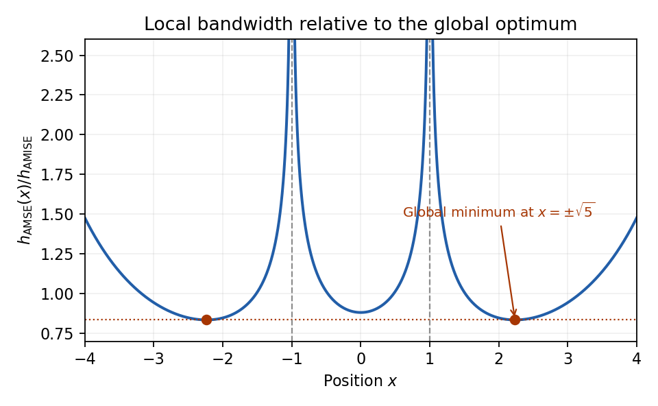
Normal-density pointwise bandwidth relative to the integrated-error optimum; minima at plus and minus square root of five
. Details. 
Let . Near the interior minimum, Taylor expansion givesOn the scale , the leading exponent is and . If the integral is localized at this minimum, the rescaled integration endpoints tend to infinity in both directions, so the Gaussian integral gives Laplace's method:Formally expanding the cubic term gives an order- correction odd in , whose Gaussian integral is zero. Quartic terms and the square of the cubic term produce the order- correction. Sufficient smoothness near the minimum and control of the exterior integral justify this formal calculation.
The printed local assumptions alone do not guarantee localization. A useful localization condition for Laplace's method is that outside each sufficiently small fixed neighbourhood of , for some , and that for some . For , the exterior contribution is at mostwhich is exponentially smaller than the displayed local term. To see why something of this kind is needed, take on . Its unique minimum is at zero and , yet on we have . This boundary interval alone contributes at least , dominating the proposed local approximation. The Laplace formula therefore has its usual implicit tail assumption, rather than following from uniqueness of the interior minimum alone.
For the gamma function, set to obtainHere has its unique minimum at , with and . It tends to infinity at both endpoints, and its integral is finite for positive exponents, so localization holds. Laplace's method yields Stirling's formula:
For a prior density and independent observations, Bayes' theorem writes the desired posterior expectation as a ratio of integrals:Suppose the log-posterior kernel has a unique concentrating interior mode , with curvature of order , and the smoothness and tail conditions hold for both integrals. Expanding quadratically gives a common Gaussian factor . Replacing the smooth amplitude by givesThis approximation does not require to be positive: it treats as an amplitude, without taking its logarithm. For more accuracy, expand the amplitude and the cubic term in the log-posterior kernel. With , the Gaussian moments are and . Terms multiplying cancel between numerator and denominator; the two remaining first corrections areunder the stronger smoothness, derivative-scaling and integrability assumptions needed for this expansion. The first term accounts for the curvature of the amplitude and the second for posterior skewness. This is posterior expectation by Laplace approximation. If there are several modes, boundary modes, or nonconcentrating tails, the appropriate separate contributions must be included; a single interior Gaussian approximation cannot then be assumed.
Articles by others on the same topic
There are currently no matching articles.