Past exam of the mathematics course of the University of Cambridge / 2016 / iii / Paper 210 (Topics in Statistical Theory)

For each ball, the event of landing in $S_j$ is a Bernoulli distribution trial. Under the null hypothesis its probability is $\epsilon$. Under the selected alternative $Q_j$, its probability is $p_1=\pi +(1-\pi )\epsilon =\epsilon +\pi (1-\epsilon )$. The placements are independent random variables conditional on that selected index, so the count has the binomial distribution:The second assertion concerns $Q_j$, rather than the unconditional mixture model $P_1$.

The Hoeffding lemma for a Bernoulli distribution variable gives $\mathbb{E}{e}^{s(B-p)}\le e^{s^2/8}$. Multiplication of the moment-generating functions of the independent random variables gives $\mathbb{E}{e}^{s(X-np)}\le e^{n{s}^2/8}$. Thus the centered count is a sub-Gaussian random variable with variance proxy $n/4$. The Chernoff bound, optimized at $s=4t/n$, givesThe same estimate holds for the lower tail by applying the Chernoff bound to $-(X-np)$. No independence between different bin counts is needed.

Put $a=\sqrt{n\log d/2}$ and $b=\sqrt{n\log (1/\delta )/2}$. Use the scan statistic $C$ and the statistical hypothesis testing ruleThe union bound and the Hoeffding inequality give $P_0(\psi =1)\le d\exp [-2(a+b{)}^2/n]\le \delta$, since $(a+b{)}^2\ge a^2+b^2$. Conditional on index $j$, accepting the null hypothesis implies $c_j\le n\epsilon +a+b$. The assumed separation gives $n\pi (1-\epsilon )>a+2b$, so this threshold lies more than $b$ below the alternative expected value $n{p}_1$. The lower-tail Hoeffding inequality therefore gives $Q_j(\psi =0)\le \delta$. Averaging the conditional error over the mixture model gives $P_1(\psi =0)\le \delta$ as well.

For $P\ll Q$, the chi-squared divergence is ${\chi }^2(P\Vert Q)={\mathbb{E}}_Q[(dP/dQ-1{)}^2]$. Write $L_j=d{Q}_j/d{P}_0$ for the likelihood ratios of the complete $n$-ball sample. Since $d{P}_1/d{P}_0=d^{-1}{\sum }_j{L}_j$ and ${\mathbb{E}}_0{L}_j=1$, the second moment of a mixture likelihood ratio givesIf instead $L_j$ denotes a one-ball likelihood ratio, its cross moment must be raised to the $n$th power for the full sample, by independence.

Let $a={\pi }^2({\epsilon }^{-1}-1)$. From the supplied second moment of a mixture likelihood ratio, dropping a nonpositive term givesThe last step uses the assumed separation. It has a real square root only when $16{\nu }^{2}d\ge 1$; otherwise no parameters satisfy it. The chi-squared testing lower bound follows from the Cauchy-Schwarz inequality: $\Vert P_1-P_0{\Vert }_{\mathrm{TV}}\le \frac{1}{2}\sqrt{{\chi }^2(P_1\Vert P_0)}\le 2\nu$. Every statistical hypothesis testing rule has sum of its Type I error and Type II error at least $1-\Vert P_1-P_0{\Vert }_{\mathrm{TV}}$. Its larger error is at least half the sum, hence

Because the scalar signal and the noise vector are independent random variables with normal distributions, their sum is a Gaussian random vector. Its expected value is zero, and the covariance matrix isThus this is a rank-one covariance spike. Each summand $X_i{X}_i^{\top }$ has expected value ${\Sigma }_S$, so $\mathbb{E}\hat{\Sigma }={\Sigma }_S$. Here the empirical matrix is an uncentered empirical second-moment matrix; because the population expected value is known to be zero, it is an unbiased estimator of the covariance matrix. The TeX's apparent factorial denominator is a transcription error.

Use the convention $\mathbb{E}{e}^{sX}\le e^{{\sigma }^2{s}^2/2}$ for the centered sub-Gaussian random variable. Applying the two-sided Chernoff bound to $X$ gives $\mathbb{P}(|X|>x)\le 2e^{-x^2/(2{\sigma }^2)}$. Since $\mathbb{E}{X}^2\ge 0$, this already supplies the requested bound:For averages of independent random variables, the stronger useful statement is that the centered square of a sub-Gaussian random variable is a sub-exponential random variable. The Bernstein bound for independent sub-exponential variables then give $\mathbb{P}(n^{-1}{\sum }_i(X_i^2-\mathbb{E}{X}_i^2)>t)\le 2\exp [-cn\min \{t^2/{\sigma }^4,t/{\sigma }^2\}]$ for a universal positive $c$. These are the concentration theorems used for quadratic scan statistics.

Put $\ell =\log (d/\delta )$ and $r=\sqrt{\ell /n}\le 1$. Use the quadratic scan statistic $\Lambda$ and reject when $\Lambda >1+4r$. Under the null hypothesis, each $nu(T{)}^{\top }\hat{\Sigma }u(T)$ has the chi-squared distribution with $n$ degrees of freedom. The chi-squared concentration inequality gives $P_0^{\otimes n}(\Lambda >1+2r+2r^2)\le d{e}^{-\ell }=\delta$, by the union bound. Since $2r+2r^2\le 4r$, the proposed Type I error is at most $\delta$.

For the true set $S$, $nu(S{)}^{\top }\hat{\Sigma }u(S)/(1+\theta )$ has the same chi-squared distribution. We need a lower-tail bound that remains positive even when $\ell /n$ is close to one. Set $a=e^{-4r}$. The chi-squared Chernoff lower-tail bound gives $P(V\le na)\le \exp [-n(a-1-\log a)/2]\le e^{-n{r}^2}=e^{-\ell }$: indeed $e^{-4r}-1+4r\ge 2r^2$ for $0\le r\le 1$. To verify this last inequality, its derivative is $4(1-r-e^{-4r})$; the expression in parentheses is strictly concave, starts at zero, and changes sign once, so the minimum occurs at an endpoint, where the inequality holds.

The function $g(r)=(1+4r)e^{4r}-1$ is convex with $g(0)=0$, so $g(r)\le rg(1)<300r$ on this interval. Consequently $\theta >300r$ implies $(1+\theta )e^{-4r}>1+4r$. Failure to reject then requires $V\le na$, giving Type II error at most $e^{-\ell }\le \delta$, uniformly in $S$. An explicit, deliberately conservative answer isThe sharp constant is unnecessary; the detection scale is $\sqrt{\log (d/\delta )/n}$.

Define $P_{\theta ,n}=d^{-1}{\sum }_{S\in \mathcal{S}}{P}_{\theta ,S}^{\otimes n}$. Expanding its chi-squared divergence by the second moment of a mixture likelihood ratio, and using the supplied one-observation cross moment and independence, givesHere $S,T$ are independent uniform members of the specified family of cyclic intervals. Their overlap $R=|S\cap T|$ does not have the hypergeometric distribution of arbitrary uniform $k$-subsets. The family's geometry must be retained.

Let $x={\theta }^2{R}^2/k^2<1/4$. Since $-\log (1-x)\le x/(1-x)\le 2x$ and $R^2/k^2\le R/k$, we obtain $(1-x{)}^{-n/2}\le e^{nx}\le e^{n{\theta }^{2}R/k}$. Taking the expected value proves the upper bound. The factor $n$ in the last exponent is present in the PDF and missing in the TeX aid.

Two independent cyclic intervals intersect with probability at most $\min \{1,(2k-1)/d\}\le 2k/d$. For $k\le d/2$, precisely the $2k-1$ starting-point offsets $-(k-1),\dots ,k-1$ can overlap; for larger $k$, the upper bound is automatic. The cyclic interval overlap bound and the preceding chi-squared divergence estimate therefore giveAs in 1(e), the square-root hypothesis is meaningful when $\alpha d\ge 1$. The chi-squared testing lower bound bounds the total variation distance by $\sqrt{2{\alpha }^{\epsilon }}/2$. The worst individual Type II error dominates the error under the uniform mixture model. ThusTaking $\alpha$ small makes this lower bound informative. This argument uses the actual cyclic-interval alternative, without substituting a different family of subsets.

Each row of the oriented incidence matrix records one signed endpoint difference, henceReversing an edge changes the sign of its row, and permuting the edges permutes rows; neither operation changes the sum of absolute differences. Thus the graph total variation is independent of the chosen orientation and ordering. If $D\theta =0$, values agree at the endpoints of every edge. Any two graph vertices of a connected graph are joined by a graph path, so their values agree. Therefore $\ker D=\mathrm{span}\{1\}$.

Let $h=\hat{\theta }-{\theta }^{\ast }$. The defining minimum for graph total variation denoising, compared with the feasible value ${\theta }^{\ast }$, gives $n^{-1}\Vert z-h{\Vert }_2^2+\lambda \Vert D\hat{\theta }{\Vert }_1\le n^{-1}\Vert z{\Vert }_2^2+\lambda \Vert D{\theta }^{\ast }{\Vert }_1$. Expand the squared Euclidean norm and cancel $\Vert z{\Vert }_2^2/n$ to obtain the basic inequality for a penalized least-squares estimator:

Decompose $h={\Pi }_{1}h+D^{†}Dh$ using the incidence pseudoinverse decomposition. The Cauchy-Schwarz inequality controls the constant component, and the duality of the ${\ell }_{\infty }$ and ${\ell }_1$ norms controls the remaining component:On the stipulated event, the second term contributes at most $\lambda \Vert Dh{\Vert }_1$ after multiplication by $2/n$. The triangle inequality gives $\Vert Dh{\Vert }_1\le \Vert D\hat{\theta }{\Vert }_1+\Vert D{\theta }^{\ast }{\Vert }_1$, so the negative penalty in the basic inequality for a penalized least-squares estimator cancels. We obtainon an event of probability at least $1-\delta$.

With the usual variance-proxy convention for a sub-Gaussian random vector, every column inner product is a sub-Gaussian random variable with proxy at most ${\tau }^2$. The two-sided Chernoff bound and union bound implywith probability at least $1-\delta$. No independence between these inner products is required.

The printed coefficient-one bound is false under this convention. Take $k=m=1$, $A=[1]$, and $g=\pm \tau$ with equal probability. This Rademacher random variable has the stipulated variance proxy, but for $\delta =0.99$ the printed threshold is less than $\tau$, whereas $|g|=\tau$ surely. Even a general sub-Gaussian assumption does not imply Gaussian concentration inequality for arbitrary Lipschitz functions. Under the stronger convention $\mathbb{E}{e}^{⟨a,g⟩}\le e^{{\tau }^2\Vert a{\Vert }_2^2/4}$, the same union bound proves the printed constants. That convention, however, differs from the binomial variance proxy used in 1(b).

Let $B_{\delta }=\sqrt{\log (2m)}+\sqrt{\log (1/\delta )}$. The columns of $D^{†}/L$ have Euclidean norm at most one. Under the usual sub-Gaussian random vector convention, 3(d) justifies the tuning choice $\lambda =2\sqrt{2}L{B}_{\delta }/n$, which is independent of ${\theta }^{\ast }$. Also $\Vert {\Pi }_{1}z{\Vert }_2=|⟨z,1/\sqrt{n}⟩|$, so the Chernoff bound gives $\Vert {\Pi }_{1}z{\Vert }_2^2\le c_{\delta }=2\log (2/\delta )$ with probability at least $1-\delta$.

On the intersection of these events, of probability at least $1-2\delta$, set $a=\Vert h{\Vert }_2/\sqrt{n}$ and $b=\Vert {\Pi }_{1}z{\Vert }_2/\sqrt{n}$. The weighted Young inequality gives $2ab\le t^2{a}^2+b^2/t^2$ for $0<t<1$. Applying it to 3(c) and rearranging yields the rigorous boundIf the coefficient-one concentration statement in 3(d) is taken as an extra hypothesis, instead choose $\lambda =2L{B}_{\delta }/n$; the identical argument gives precisely the printed coefficient $4$ in the first term. Thus the deterministic argument and its risk rate are sound; its concentration constants depend on correcting or strengthening 3(d).

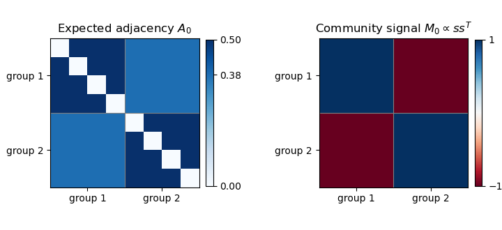
Write $s_i=1$ on $S$ and $s_i=-1$ on $S^c$, and put $v=s/\sqrt{n}$ and $w=1/\sqrt{n}$. Because the two groups have equal size, $v,w$ are orthonormal. Let $a=1/2-t/(2\sqrt{n})$ and $b=t/(2\sqrt{n})$. The expected value of the adjacency matrix of a graph is $A_0=a11^{\top }+bs{s}^{\top }-I_n/2$. ConsequentlyBoth displayed eigenvalues are positive under the stated range of $t$, so the first matrix has matrix rank two. The other $n-2$ eigenvalues are zero. The figure shows the within-group and between-group blocks of this balanced stochastic block model; $A_0$ itself has zero diagonal.

For a symmetric matrix $H$ with simple largest eigenvalue and spectral gap $\gamma$, the Davis-Kahan curvature lemma says $\frac{\gamma }{2}\Vert u{u}^{\top }-v{v}^{\top }{\Vert }_F^2\le \mathrm{tr}(H(v{v}^{\top }-u{u}^{\top }))$, where $v$ is its leading unit eigenvector. Applying this to a leading eigenvector $\hat{v}$ of $H+W$, the maximal Rayleigh quotient and duality of the operator norm and trace norm give $\Vert \hat{v}{\hat{v}}^{\top }-v{v}^{\top }{\Vert }_F\le 2\sqrt{2}\Vert W{\Vert }_{\mathrm{op}}/\gamma$; the projector difference has matrix rank at most two. This is a rank-one eigenprojector perturbation bound.

Here $W=M-M_0=A-A_0$ has independent centered bounded upper-triangular entries, apart from symmetry. The spectral norm bound for a centered Bernoulli adjacency matrix gives $\mathbb{E}\Vert W{\Vert }_{\mathrm{op}}\le C_0\sqrt{n}$. Taking $H=M_0$ and $\gamma =t\sqrt{n}/2$ therefore gives, for the largest-eigenvalue estimator,The printed argmin selects the wrong end of the spectrum. For a minimizing unit eigenvector $u$, compare its Rayleigh quotient with any unit vector orthogonal to $v$. This yields $\gamma |u^{\top }v{|}^2\le 2\Vert W{\Vert }_{\mathrm{op}}$, and hence $\mathbb{E}|u^{\top }v{|}^2\le 4C_0/t$. Its mean projector error is at least $\sqrt{2}(1-4C_0/t)$, using $\sqrt{1-x}\ge 1-x$. Along $t=n^{1/4}$ with sufficiently large even $n$, the printed parameter restriction holds and this lower bound tends to $\sqrt{2}$, contradicting an error of order $1/t$. Replace argmin by argmax, or negate the entire matrix before minimizing.

For partitions, the appropriate Hamming distance between unlabelled bipartitions is $\Delta (T,S)=\min \{|T△S|,|T△S^c|\}$. It counts vertices assigned to the wrong group after the better global exchange of the two group names. The printed signed-indicator formula does not implement this exchange: negating a zero-one indicator is not taking its complement. It must be read as this partition distance, or written with the $\pm 1$ membership vectors.

Use the corrected leading eigenvector estimator from 4(b), and orient its sign to minimize $\Vert \hat{v}-\sigma v{\Vert }_2$. At every wrongly signed coordinate, this difference has magnitude at least $1/\sqrt{n}$. Therefore the sign rounding bound for a unit eigenvector givesThe last inequality uses the projector distance bound $\sqrt{2}\le 2$. Taking the expected value of this Frobenius norm estimate proves $\mathbb{E}\Delta (\hat{S},S)\le 2nc/t$. The assertion relies on the corrected estimator and partition-distance definition.

The Kullback-Leibler divergence of a product measure is the sum of the individual divergences, by expanding the logarithm of the likelihood ratio and taking its expected value. Put $q=1/2-t/\sqrt{n}$ and define $W(S)$ to be the unordered pairs lying within one group, while $C(S)$ is the set of unordered pairs crossing between groups. ThenThus choosing the printed $\partial S$ to mean $W(S)$ gives its order of the summands. If $\partial S$ denotes the usual graph cut $C(S)$, their two orders must be interchanged. Each unordered edge is counted once.

The inequality $\log x\le x-1$ givesSince $1/3<q<1/2$, each changed-edge divergence is at most $9t^2/(2n)$. Summing over at most $n(n-1)/2$ pairs gives $D_{\mathrm{KL}}(P_S\Vert P_{S^{\prime }})\le 9n{t}^2/4$. This is the information scale needed for Fano's inequality.

In natural logarithms, Fano's inequality for a uniform index $J$ among $N$ alternatives states $\mathbb{P}(\hat{J}\ne J)\ge 1-(I(J;G)+\log 2)/\log N$. The mutual information is at most the average Kullback-Leibler divergence to any fixed reference law. With the supplied packing, nearest-neighbour decoding turns partition error below half the separation into correct decoding. Thus the packing alone proves a bound at radius $n(1/4-\epsilon /2)$, with the unavoidable $\log 2$ term. It does not automatically prove the much larger printed radius.

A list-decoding Fano inequality supplies the intended near-half error threshold. Assume $0<\epsilon <1/4$, since otherwise that threshold is nonpositive and its event is automatic. Take a uniform prior on all $N=\left(\genfrac{}{}{0ex}{}{n}{n/2}\right)/2$ unlabelled balanced partitions, and let $r=n(1/2-2\epsilon )$. A Hamming ball of radius less than $r$ around any estimated partition contains at most $B={\sum }_{j<r}\left(\genfrac{}{}{0ex}{}{n}{j}\right)$ such partitions. This follows by selecting the representative closer to the estimated group; each unlabelled partition contributes at most one such representative because $r<n/2$. The entropy bound for a Hamming ball gives $\log B\le nh(r/n)$, where $h$ is the binary entropy function measured in natural logarithms. Its curvature gives $\log 2-h(1/2-2\epsilon )\ge 8{\epsilon }^2$. Also $\left(\genfrac{}{}{0ex}{}{n}{n/2}\right)\ge 2^n/(n+1)$, soUse the all-$1/2$ independent-edge law $P_{\ast }$ as a reference. Only the $n^2/4$ crossing pairs differ; the preceding Bernoulli distribution divergence estimate gives $D_{\mathrm{KL}}(P_S\Vert P_{\ast })\le n{t}^2$. Hence $I(J;G)\le n{t}^2$. Whenever the denominator is positive, the list-decoding Fano inequality proves the finite-sample answerFor $4{\epsilon }^{2}n\ge \log (2(n+1))$, this is at least $1-t^2/(4{\epsilon }^2)-\log 2/(4{\epsilon }^{2}n)$. If in addition $n{t}^2\ge \log 2$, it implies the intended form with $c^{\prime }=1/2$. This proves the claimed information-theoretic scale with its needed finite-sample qualifications.

As a uniform finite-sample assertion for every positive $t$, the printed form is false. At $t=0$ every partition has the same data law, and a uniformly random balanced guess has a positive chance of being correct, giving error strictly below one. Such randomness can also be extracted from the finite graph sample: assign distinct graph outcomes to the finitely many balanced partitions; under the common law every selected outcome has positive probability. The worst error remains strictly below one for sufficiently small positive $t$, by continuity. The printed lower bound tends to one as $t\downarrow 0$ for any fixed universal $c^{\prime }$, which contradicts this. The entropy correction cannot be dropped without an asymptotic or signal-size condition.