By Euler's formula, . Factoring out the half-angle givesSince , the cosine is positive. ThereforeOn the Argand diagram, the points form a rhombus. Its diagonal from to bisects the angle between the unit vectors and , so its direction is ; resolving either side along the diagonal gives its length .
Similarly,Thus, for ,At , , whose complex argument is undefined. Geometrically, is the chord joining the two unit-circle points and . The isosceles triangle with vertex angle has half-chord , and the chord direction is perpendicular to the radius through its midpoint, giving the stated argument.
Componentwise,soRepeated application gives . Transposing the matrix exponential term by term therefore yieldsMultiplication of the two power series givesHenceIf is an orthogonal matrix for every real , thenIts coefficient of must vanish, sothat is, is a skew-symmetric matrix.
Because is a monotone sequence, every one of its first terms is at most , soOn the other hand, every term from through is at least , and henceBoth the lower bound and upper bound tend to because the Cesaro means converge to . The squeeze theorem gives
Convergence at implies that the terms form a bounded sequence: for some . If and , thenComparison with the convergent geometric series proves absolute convergence. The case is vacuous.
The radius of convergence is the number such that a power series converges absolutely for and diverges for , with boundary behavior considered separately.
TakeThen is the convergent alternating harmonic series, whereas is the divergent harmonic series. Thus converges at a point of modulus one and diverges at another point of modulus one. It follows that
The cross product is the vector perpendicular to and , of magnitude and orientation fixed by the right-hand rule. In suffix notation,where is the Levi-Civita symbol. ThereforeUsinggivesHence the vector triple product identity is
The identity in part (a), together with , givesFor every , is perpendicular to , because it is a scalar multiple of . ThereforeAlso and . Induction using the two-step recurrence yields
The recurrence shows that every odd-indexed position vector is a scalar multiple of , while every positive even-indexed position vector is a scalar multiple of . HenceMoreover , so these two straight lines through the origin are perpendicular.
Let be the direction vector of the segment . Consecutive vectors are perpendicular and . Using ,Thus adjacent segments are perpendicular. AlsosoIf , the norm formula in part (i) gives . If , then : the points repeat cyclically and form a square centered at the origin.
Put and choose perpendicular unit vectors such that and . Direction vectors for the two lines areandTheir scalar product and norms giveTherefore the acute angle between the straight lines satisfies
A matrix and its matrix transpose have the same characteristic polynomial, becauseThus they have the same eigenvalues, including algebraic multiplicities.
The proposed sum identity is false. Forboth eigenvalues are zero, whereashas eigenvalues . HenceEquivalently, the two sides are generally and , which need not agree.
If , then , and hence . Also because . Thus and are linearly independent eigenvectors with eigenvalue one.
For every vector ,so is nonzero but has square zero:Consequently all three eigenvalues are one. The eigenspace iswhich has dimension two. It cannot supply three linearly independent eigenvectors, so
Multiplication givesThe vector is an eigenvector with eigenvalue one. On the plane spanned by the orthonormal pair , the matrix isIts eigenvalues are the roots of , namelyFor either root, an eigenvector is . ThereforeThese positive eigenvalues are the squared singular values of .
Conversely, suppose for every real . Taking gives . Taking then gives . Thus every entry satisfies , and
A real skew-symmetric matrix satisfies , so it is a skew-Hermitian matrix. If , thenTaking the complex conjugate and using shows that this scalar is the negative of its conjugate. Henceso every eigenvalue is purely imaginary or zero.
The plane is invariant under , because . On this two-dimensional plane, is perpendicular to . Put with . Then is parallel to , andsoThe matrix exponential fixes the kernel vector:Separating even and odd powers in its series and using givesThus acts as a rotation through angle on and fixes its axis .
Write . From the coordinate formula for the cross product,If , this becomesThus gives rank three and a zero-dimensional kernel, while gives rank one and kernel dimension two.
If , then . When , the equations force and , soWhen , again and . These dimensions also agree with the rank-nullity theorem.
First computeThe vector lies in the kernel of , since . If is solvable, multiplying by gives the necessary compatibility conditionTherefore
The intermediate value theorem states that if is continuous and lies between and , then there exists such that .
A function is differentiable at when the finite limitexists. A derivative need not be continuous. For example,is differentiable everywhere and , but for ,which has no limit at zero.
Set . ThenThe extreme value theorem gives a minimum of on . If it occurs in , the two-sided difference quotient gives . If it occurs at , either or a negative right derivative contradicts minimality; the endpoint is analogous. Hence some satisfiesThis proves the Darboux theorem for derivatives in the stated case without assuming that is continuous.
Because a differentiable function is continuous, defineThe fundamental theorem of calculus gives . At the endpoints,whileApplying the result just proved to yields with
The function is continuous at when for every there is a such thatSuppose has a local minimum at and is differentiable there. For sufficiently small ,Both one-sided limits equal , so it is both nonnegative and nonpositive. Therefore
The upper bound follows immediately from convexity, sinceFor the lower bound, writeApplying convexity and rearranging givesChoose a fixed with . Applying these bounds with and shows that the difference is trapped between quantities of order . Both tend to zero, so every convex function on an open interval is continuous.
Now suppose is a local minimum but some satisfies . For sufficiently small , the point lies in the neighbourhood on which is minimal, whereas convexity givesa contradiction. ThusDifferentiability at the minimizer is unnecessary: is convex, has its global minimum at , and is not differentiable there.
For each , monotonicity gives the dyadic-block boundsSumming the upper bounds proves convergence of whenever converges. Summing the lower bounds gives, up to the first term,so convergence of forces convergence of the condensed series. This is the Cauchy condensation test:
If , the terms do not tend to zero, so the series diverges by the term test for divergence. If , the terms form a nonnegative decreasing sequence, and the Cauchy condensation test gives the condensed seriesThis geometric series converges exactly when . Hence the p-series criterion is
For ,Thus for all sufficiently large the ratio is, for example, at most . Comparison with a decaying geometric sequence, equivalently the ratio test, yields
We first prove by induction thatIt holds for , and if it holds at , thenConsequentlyPart (c) and the squeeze theorem now give
Let be the supremum of all lower Darboux sums and the infimum of all upper Darboux sums. The assumed comparison of arbitrary lower and upper sums gives . For the partition supplied for a given ,Since this holds for every positive , . Thus the Riemann integrability criterion gives
If is continuous on , the Heine-Cantor theorem makes it uniformly continuous. Given , choose so that intervals of length below have oscillation below . A partition of mesh below then satisfiesproving that Continuous functions are Riemann integrable.
For the function defined using , choose with . Given , choose so small that . On , the function is continuous and therefore has a partition whose upper-minus-lower sum is below . Adding the interval contributes at most , regardless of the value . Hence the full Darboux-sum difference is below , and
Finally, for any partition , the mean value theorem supplies such thatSumming telescopes toa Riemann sum for the Riemann-integrable function . Equivalently, every lower derivative sum is at most this telescoping value and every upper derivative sum is at least it. Taking the common upper and lower Darboux integrals proves the fundamental theorem of calculus conclusion
Subtract successive terms and use a telescoping series:Thus the linear recurrence relation has solution
Put , so the same definition includes . Since and every is nonzero,The factor is a discrete integrating factor for this variable-coefficient affine recurrence. Sum the increments as a telescoping series and multiply back by :The identity requires no assumption that the coefficients have the same sign.
The first partial derivatives areBoth vanish at , so every positive diagonal point is a stationary point. The Hessian matrix there isIts eigenvectors and have respective eigenvaluesThe zero eigenvalue reflects the entire line of nonisolated stationary points: . In fact , showing a non-strict local minimum when , a non-strict local maximum when , and values on both sides of two near . At that last point the whole Hessian matrix vanishes, so its signs alone cannot classify the point.
Because is a nonnegative integer, its indicator function satisfies . Taking expected values proves the upper bound. The finite second moment also gives a finite expected value, by the Cauchy-Schwarz inequality. Applying that inequality to and givesThe assumed positive second moment permits division, yieldingThe lower bound is the basic second moment method; the upper bound also follows from Markov's inequality at threshold one. Integer-valuedness is essential for that upper bound, but not for the lower bound. For example, a constant would violate the upper bound.
Integrate the joint probability density over to obtain the marginal density of :Thus has an exponential distribution of rate one. Dividing the joint probability density by this marginal density gives the conditional densityEquivalently, has an exponential distribution of rate . The value at can be assigned arbitrarily: it is a probability-zero conditioning value and the density ratio there is not meaningful.
The conditional density givesusing either integration by parts or the expected value of an exponential distribution. HenceThis is a finite value for almost every realization of , but not an integrable random variable: . Since , its conditional expectation remains well-defined in the nonnegative, extended-expectation sense; the tower property of conditional expectation then gives .
With no electrical resistance or applied electric potential difference, divide the equation by the inductance to get a simple harmonic oscillator with angular frequency . Its general real solution isEach nonzero solution has period . Here is an angular frequency; the ordinary frequency in cycles per unit time is .
The PDF gives , the Heaviside step function; the TeX incorrectly changes this to . A unit voltage step has derivative the Dirac delta function, so the current is the causal Green function for .
The current must be continuous at zero: a jump would create a delta derivative through , absent on the right-hand side. Integrating across zero therefore gives , so and . PutThese distinct negative characteristic roots give the overdamped RLC responseTogether with for , this solves the step response. The eventual current is zero: the capacitor charges and blocks steady current in the series RLC circuit.
First construct the periodic response required in the introductory clause. At , the terms cancel for a sinusoid, leaving . ThusThis resonant series RLC response dissipates energy through Joule heating. Over one period,The Q factor, using the maximum magnetic energy , is consequently
Every solution is the resonant series RLC response plus a solution of the homogeneous damped harmonic oscillator. Define and . The three possibilities areThese are respectively the underdamped RLC response, critically damped RLC response and overdamped RLC response. Both exponents in the last case are negative because . All three homogeneous contributions tend to zero as , so every response approaches the unique periodic steady current . No initial conditions were specified in this clause; they determine .
Use the complete system in the PDF: the TeX omits . Both coordinate axes are invariant, and the equilibrium points are , and . The Jacobian matrix isAt its eigenvalues are , and at they are : both points are saddle equilibria. At the coexistence point,Thus the interior point is a stable spiral. The nontrivial nullclines are and : increases below the first and decreases above it, while increases to the right of the second and decreases to the left. The rotation near coexistence is counterclockwise.
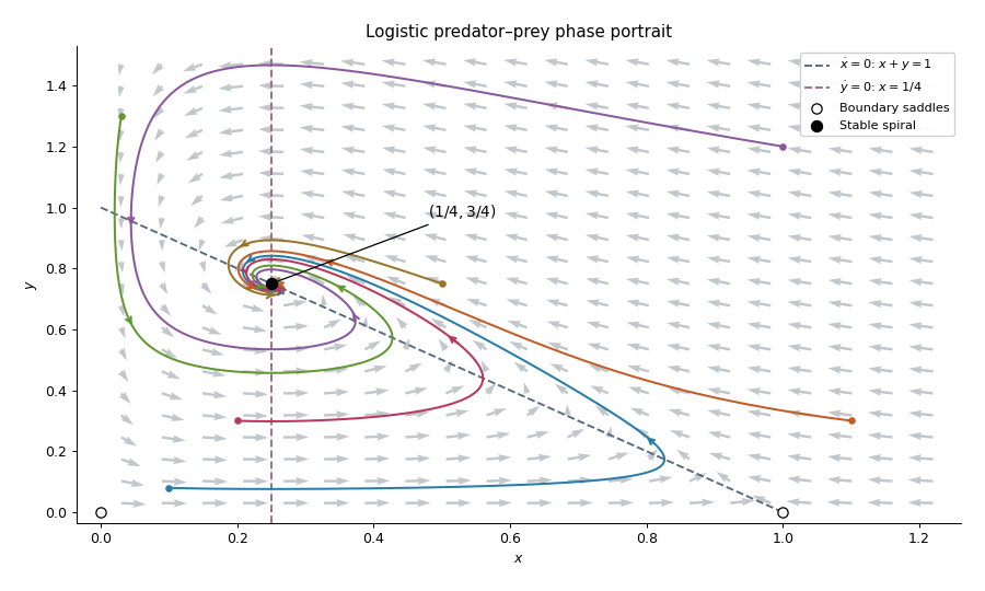
Trajectories of a predator-prey system
. A local linearization by itself does not prove that every interior solution has the same limit. For this logistic predator-prey model, let and use the Lyapunov functionThe inequality makes nonnegative, with equality only at coexistence. Its sublevel sets are compact inside the positive quadrant, because diverges both at the axes and at infinity. Direct differentiation cancels the predator-prey cross terms and givesOn one has , and remaining there requires . The largest invariant subset is therefore the coexistence point. The LaSalle invariance principle provesOn , decays as toward the origin. On , the logistic differential equation takes every to one. The origin itself stays fixed. These boundary trajectories are the exceptions to the interior convergence statement.
For , differentiate and use the angular derivative . The polar coordinates satisfyHence the rotation is clockwise. The origin is an unstable equilibrium, while is a limit cycle of period . Writing gives the logistic differential equation . For ,All nonzero solutions tend to the unit-circle attracting limit cycle as , spiralling outward for and inward for . For the solution exists for every real time and approaches the origin as ; for it remains periodic in both time directions. For , the denominator first vanishes atThis finite-time blow-up of an ordinary differential equation occurs backward in time. Such exterior solutions have no behavior: their maximal time interval is . The zero solution exists for all time and has no defined polar angle.
Articles were limited to the first 100 out of 256 total.
Articles by others on the same topic
There are currently no matching articles.