Subtract successive terms and use a telescoping series:Thus the linear recurrence relation has solution
Put , so the same definition includes . Since and every is nonzero,The factor is a discrete integrating factor for this variable-coefficient affine recurrence. Sum the increments as a telescoping series and multiply back by :The identity requires no assumption that the coefficients have the same sign.
The first partial derivatives areBoth vanish at , so every positive diagonal point is a stationary point. The Hessian matrix there isIts eigenvectors and have respective eigenvaluesThe zero eigenvalue reflects the entire line of nonisolated stationary points: . In fact , showing a non-strict local minimum when , a non-strict local maximum when , and values on both sides of two near . At that last point the whole Hessian matrix vanishes, so its signs alone cannot classify the point.
Because is a nonnegative integer, its indicator function satisfies . Taking expected values proves the upper bound. The finite second moment also gives a finite expected value, by the Cauchy-Schwarz inequality. Applying that inequality to and givesThe assumed positive second moment permits division, yieldingThe lower bound is the basic second moment method; the upper bound also follows from Markov's inequality at threshold one. Integer-valuedness is essential for that upper bound, but not for the lower bound. For example, a constant would violate the upper bound.
Integrate the joint probability density over to obtain the marginal density of :Thus has an exponential distribution of rate one. Dividing the joint probability density by this marginal density gives the conditional densityEquivalently, has an exponential distribution of rate . The value at can be assigned arbitrarily: it is a probability-zero conditioning value and the density ratio there is not meaningful.
The conditional density givesusing either integration by parts or the expected value of an exponential distribution. HenceThis is a finite value for almost every realization of , but not an integrable random variable: . Since , its conditional expectation remains well-defined in the nonnegative, extended-expectation sense; the tower property of conditional expectation then gives .
With no electrical resistance or applied electric potential difference, divide the equation by the inductance to get a simple harmonic oscillator with angular frequency . Its general real solution isEach nonzero solution has period . Here is an angular frequency; the ordinary frequency in cycles per unit time is .
The PDF gives , the Heaviside step function; the TeX incorrectly changes this to . A unit voltage step has derivative the Dirac delta function, so the current is the causal Green function for .
The current must be continuous at zero: a jump would create a delta derivative through , absent on the right-hand side. Integrating across zero therefore gives , so and . PutThese distinct negative characteristic roots give the overdamped RLC responseTogether with for , this solves the step response. The eventual current is zero: the capacitor charges and blocks steady current in the series RLC circuit.
First construct the periodic response required in the introductory clause. At , the terms cancel for a sinusoid, leaving . ThusThis resonant series RLC response dissipates energy through Joule heating. Over one period,The Q factor, using the maximum magnetic energy , is consequently
Every solution is the resonant series RLC response plus a solution of the homogeneous damped harmonic oscillator. Define and . The three possibilities areThese are respectively the underdamped RLC response, critically damped RLC response and overdamped RLC response. Both exponents in the last case are negative because . All three homogeneous contributions tend to zero as , so every response approaches the unique periodic steady current . No initial conditions were specified in this clause; they determine .
Use the complete system in the PDF: the TeX omits . Both coordinate axes are invariant, and the equilibrium points are , and . The Jacobian matrix isAt its eigenvalues are , and at they are : both points are saddle equilibria. At the coexistence point,Thus the interior point is a stable spiral. The nontrivial nullclines are and : increases below the first and decreases above it, while increases to the right of the second and decreases to the left. The rotation near coexistence is counterclockwise.
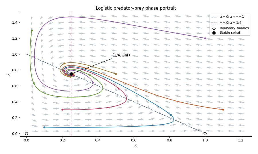
Trajectories of a predator-prey system
. A local linearization by itself does not prove that every interior solution has the same limit. For this logistic predator-prey model, let and use the Lyapunov functionThe inequality makes nonnegative, with equality only at coexistence. Its sublevel sets are compact inside the positive quadrant, because diverges both at the axes and at infinity. Direct differentiation cancels the predator-prey cross terms and givesOn one has , and remaining there requires . The largest invariant subset is therefore the coexistence point. The LaSalle invariance principle provesOn , decays as toward the origin. On , the logistic differential equation takes every to one. The origin itself stays fixed. These boundary trajectories are the exceptions to the interior convergence statement.
For , differentiate and use the angular derivative . The polar coordinates satisfyHence the rotation is clockwise. The origin is an unstable equilibrium, while is a limit cycle of period . Writing gives the logistic differential equation . For ,All nonzero solutions tend to the unit-circle attracting limit cycle as , spiralling outward for and inward for . For the solution exists for every real time and approaches the origin as ; for it remains periodic in both time directions. For , the denominator first vanishes atThis finite-time blow-up of an ordinary differential equation occurs backward in time. Such exterior solutions have no behavior: their maximal time interval is . The zero solution exists for all time and has no defined polar angle.
Assume the usual continuous-coefficient setting for a second-order linear differential equation. The Wronskian has derivativewhich proves the Abel identity. If , the two initial-value columns are linearly dependent, so some nonzero gives and . The uniqueness theorem for ordinary differential equations makes that linear combination identically zero. If , the initial-value matrix is an invertible matrix, givingThis establishes the alternative and supplies any prescribed initial data.
For the Airy ordinary differential equation, substitute a power series . Coefficient comparison gives andChoose and . The Airy power-series fundamental pair isEmpty products mean one. Their first terms are and . The ratio test gives convergence for every finite , so termwise differentiation verifies the equation. Their Wronskian is one at zero, and hence everywhere because . Thus every solution is .
For real initial data, separation of variables givesThis includes , whose solution is identically zero. Every other real has a pole at , so only gives a finite solution on the whole real line. If complex-valued initial data are allowed, a nonreal has no real-time pole; the whole-real-line conclusion here uses the usual real-valued differential-equation convention.
Along a characteristic curve , the chain rule gives . For the homogeneous transport equation this is zero, so . For the nonlinear equation, the same method of characteristics reduces the problem to , with initial value . ThereforeFor differentiable real , this is the classical solution wherever its denominator is nonzero, on the characteristic intervals containing the initial line. If for some , that characteristic blows up at , . Thus the only real-valued solution bounded on all of has , giving .
Choose and , so . The Jacobian determinant of the coordinate change is two, so it is an invertible linear map. By the chain rule, and . ConsequentlyThis is the wave equation with . The D'Alembert formula is , with arbitrary twice differentiable functions . Returning to the old coordinates and absorbing factors of two into the arbitrary functions givesDirect differentiation checks the cancellation. Equivalently, first integrating produces the same two-function family.
The binomial theorem makes the sum of the proposed probability mass function equal to ; every term is nonnegative. Realize the associated binomial distribution as , where the are independent variables with the Bernoulli distribution of parameter . Each has expected value and variance . Linearity of expectation and variance additivity for independent random variables yieldAt or this is a constant random variable; the same formulas apply, with the endpoint mass understood by continuity.
For fixed and sufficiently large ,The finite product and last factor tend to one, while . Thus the Poisson limit theorem givesThese numbers form a probability mass function because they are nonnegative and their sum is , by the exponential series. They define the Poisson distribution of parameter . Only is needed to make the binomial parameter valid, which is sufficient for the limit.
Let and use the floor function to chooseInterpret an empty integer interval as an empty sum. These bounds give exactly the event , where has the binomial distribution of parameters . Since , the central limit theorem for a sum of independent Bernoulli distribution variables gives convergence in distribution of that standardized count to the standard normal distribution. Its cumulative distribution function is continuous at both endpoints, soThe TeX's additional malformed inequality involving and is absent from the PDF and is not a condition on the requested integers.
Apply Markov's inequality to the nonnegative random variable , since implies :This exponential Markov bound remains true, though uninformative, when the expected value is infinite. For a standard normal distribution, completion of the square gives its moment-generating functionMinimize over positive ; the choice gives the Chernoff bound
Use the rate convention for the exponential distribution. By convolution of independent random variables, the probability density function of is, for ,It is zero for . The expression is nonnegative whichever rate is larger, and defines a two-stage hypoexponential distribution. As a check, its limit as is , the shape-two gamma distribution.
For , independence gives the survival function for . Differentiating its complement givesThus the minimum has an exponential distribution whose rate is the sum of the rates.
Use the positive exponent in the PDF. The TeX introduces a minus sign in the numerator while retaining the positive-sign normalizing constant, which would not define the stated probability distribution. The Curie–Weiss model assigns equal weights to and , since is unchanged by simultaneous reversal. This spin inversion symmetry pairs every configuration with one having the opposite value of , so
Let , using the supplied correlation property of the Curie–Weiss model. Since and each spin has zero expected value,Divide by to obtainThe expression assumes , as required for to exist. It makes the connection between the spin correlation and the requested conditional probability explicit.
If exactly spins equal , then . Therefore its possible values are , with for . Choosing the positive spins gives the binomial coefficientEvery such configuration has the same Curie–Weiss model weight because . The probability mass function of this spin magnetization is consequentlyand zero elsewhere. Grouping the original partition function by the same count also giveswhich verifies normalization without counting any configuration twice.
Write and . The expected duration of symmetric gambler's ruin satisfies and, by conditioning on the first step,These expected values are finite: from any interior state, consecutive right steps ensure absorption, an event of probability at least . Blocks of steps therefore bound the survival probability by a decreasing geometric sequence. The candidate has the required boundary values and satisfies . HenceFor completeness, the difference of two solutions of this linear recurrence relation has zero second difference and is affine in ; its two zero boundary values force it to vanish.
The vertices visited by a simple symmetric random walk form an integer interval: nearest-neighbour steps cannot skip a vertex. At the stopping time , write that interval as , with . The walk is at one of its endpoints, because the th new vertex must extend the earlier interval. This also covers , when both endpoints coincide.
The Strong Markov property restarts the walk from this endpoint. Visiting a new vertex is exactly exiting , or reaching or . Translate these absorbing boundaries to . The starting point becomes either or , so the expected duration of symmetric gambler's ruin is in both cases. Taking conditional expectations and then expected values gives the expected time to expand a random-walk range:
Couple the walk on the cycle graph to a simple symmetric random walk on the integer line by taking , using the same increments. The visited integer interval has distinct residues until its length reaches ; an interval of exactly consecutive integers contains every residue once. Consequently the cover time on the cycle is exactly in this coupling.
Since , telescope the range-expansion times and use linearity of expectation, without assuming those times are independent:This is the expected cover time of a cycle. The restriction makes the two neighbours distinct, matching the supplied transition rule.
Articles by others on the same topic
There are currently no matching articles.