Past exam of the mathematics course of the University of Cambridge / 2017 / ia / Paper 4

Reduce $z$ using modular congruence: its residue class modulo $3$ is $0$, $1$, or $-1$. A square number therefore has residue class $0$ or $1$, and raising either residue to the positive integer power $n$ leaves it unchanged. ConsequentlyThe exponent in the original PDF is $2n$; the polynomial identities in the converted TeX are a transcription error. The argument uses $n\ge 1$; it does not assign $0^0$ a value.

For a Pythagorean triple, each square number is $0$ or $1$ modulo $3$. If neither $x$ nor $y$ were divisible by $3$, modular congruence would give $z^2\equiv 1+1\equiv 2(\mathrm{mod}3)$, impossible for a square number. Thus at least one of $x,y$ is divisible by $3$; both can be divisible, as in $(9,12,15)$.

An odd number has square number congruent to $1$ modulo $4$, whereas an even number has square number congruent to $0$. If both $x$ and $y$ were odd numbers, their sum of square numbers would again be $2$ modulo $4$, which no square number can be. Hence $x$ and $y$ cannot both be odd. They can both be even; the conclusion does not require the Pythagorean triple to be primitive.

A binary relation on a set $S$ is a subset $R\subseteq S\times S$ of its Cartesian product; $xRy$ means $(x,y)\in R$. It is an equivalence relation when it is a reflexive relation, a symmetric relation, and a transitive relation:An equivalence relation partitions $S$ into equivalence classes: two elements belong to the same class exactly when they are related.

The first condition concerns the domains: their symmetric difference $A△B$ must be a finite set. The original PDF prints this condition and the agreement condition together; the converted TeX omits both. The two existing solution scopes are used here to prove the domain and value parts of the single equivalence relation assertion.

Domain agreement is a reflexive relation because $A△A=\varnothing$, and a symmetric relation because $A△B=B△A$. For the transitive relation property, membership can differ between $A$ and $C$ only if it differs between $A$ and $B$ or between $B$ and $C$. ThusA set union of two finite sets is finite, so the domain condition passes through a chain of related pairs. This is the domain part of equivalence of partial functions modulo finite changes.

For the value condition, a function agrees with itself outside the empty exceptional set, proving the reflexive relation property. Interchanging the two functions preserves equality, so the same exceptional finite set proves the symmetric relation property.

Suppose $(A,f)$ is related to $(B,g)$ and $(B,g)$ to $(C,h)$, with exceptional finite sets $F_{AB}$ and $F_{BC}$. Points of $A\cap C$ might be absent from $B$, so merely taking $F_{AB}\cup F_{BC}$ would miss a real issue. Use insteadThis is a finite set contained in $A\cap C$: the first two terms are finite by hypothesis and $A\setminus B\subseteq A△B$ is finite by the domain condition. If $x\in (A\cap C)\setminus F_{AC}$, then $x\in B$ and neither original exception occurs, so $f(x)=g(x)=h(x)$. The domain condition is also preserved, as proved in the preceding scope. Thus the full relation is a transitive relation, andFinite domains cause no problem: one may take the whole intersection as the exceptional set. Both conditions are needed for equivalence of partial functions modulo finite changes.

Assume the particle masses $m_i$ are fixed and their total mass $M={\sum }_i{m}_i$ is positive. The centre of mass and the relative position vectors areTheir weighted sum is zero, so differentiation gives ${\sum }_i{m}_i{\dot{\mathbf{y}}}_i=0$. Expanding the kinetic energy with ${\dot{\mathbf{x}}}_i=\dot{\mathbf{R}}+{\dot{\mathbf{y}}}_i$ makes the mixed term vanish:This kinetic-energy decomposition about the centre of mass separates translation from internal motion without assuming any particular force law.

For the rigid body, its relative velocity is ${\dot{\mathbf{y}}}_i=\omega \mathbf{n}\times {\mathbf{y}}_i$. The cross product identity for a unit vector gives $|\mathbf{n}\times {\mathbf{y}}_i{|}^2=|{\mathbf{y}}_i{|}^2-(\mathbf{n}\cdot {\mathbf{y}}_i{)}^2$, the squared perpendicular distance to the rotation axis. Hence the moment of inertia of the particle is $I_i=m_i[|{\mathbf{y}}_i{|}^2-(\mathbf{n}\cdot {\mathbf{y}}_i{)}^2]$, and summing the rotational kinetic energy yields

The dimensions are $[m]=\mathsf{M}$, $[\alpha ]=\mathsf{M}{\mathsf{T}}^{-1}$, $[u_0]=\mathsf{L}{\mathsf{T}}^{-1}$, and $[g]=\mathsf{L}{\mathsf{T}}^{-2}$. Under the stated model, $m,\alpha ,u_0,g$ are the only parameters determining the ascent time. If $m^p{\alpha }^q{u}_0^r{g}^s$ is dimensionless, then $p+q=0$, $r+s=0$, and $-q-r-2s=0$, leaving one independent dimensionless variable. One convenient choice isThus dimensional analysis fixes the form, but Newton's second law must determine the function $f$.

Take upward velocity as positive. Throughout ascent, Newton's second law with linear drag gives $m\dot{v}=-mg-\alpha v$. An integrating factor or direct solution of this linear ordinary differential equation givesThe first zero of this velocity is the highest point, soThis vertical ascent under linear drag has $T<u_0/g$ for $u_0>0$, since $\log (1+\lambda )<\lambda$. The limit $\alpha \to 0$ recovers the no-drag ascent time $u_0/g$; $u_0=0$ gives $T=0$.

The Fermat-Euler theorem states that for an integer $a$ and a positive integer $n$ with $\gcd (a,n)=1$,where the Euler totient function $\phi (n)$ counts the residue classes coprime to $n$. For $n\ge 2$, choose a reduced residue system $r_1,\dots ,r_{\phi (n)}$. Multiplication by the unit modulo n $a$ preserves coprimality and is injective on these residue classes: $a{r}_i\equiv a{r}_j(\mathrm{mod}n)$ implies $r_i\equiv r_j(\mathrm{mod}n)$, because $a$ has a multiplicative inverse modulo $n$. It therefore permutes the reduced residue system, givingThe product is also a unit modulo n, so it can be cancelled. This proves the Fermat-Euler theorem. For $n=1$ every modular congruence is automatic; one may use $\phi (1)=1$.

For a prime number $p$, the Euler totient function has value $\phi (p)=p-1$. Thus $a^{p-1}\equiv 1(\mathrm{mod}p)$ whenever $p\nmid a$. Multiplying by $a$, and treating $p\mid a$ separately, gives the all-integer version of Fermat's little theorem:Finally, Wilson theorem states that for every prime number $p$, $\boxed{(p-1)!\equiv -1(\mathrm{mod}p)}$. Its converse is also true: an integer $n>1$ is prime exactly when $(n-1)!\equiv -1(\mathrm{mod}n)$. For the converse, any proper divisor $1<d<n$ would divide both $(n-1)!$ and $n$, contradicting that congruence.

Suppose $X^2\equiv -1(\mathrm{mod}p)$. Then $X$ is a unit modulo n for modulus $p$, and Fermat's little theorem impliesSince $p$ is an odd prime number, $1$ and $-1$ are distinct residue classes. Therefore $(p-1)/2$ is even, and $p\equiv 1(\mathrm{mod}4)$.

Conversely, put $q=(p-1)/2$. Pair each integer $j\in \{1,\dots ,q\}$ with $p-j$ in the factorial. Wilson theorem yieldsWhen $p\equiv 1(\mathrm{mod}4)$, $q$ is even, so $X=q!$ satisfies $X^2\equiv -1(\mathrm{mod}p)$. This proves the first supplementary law for quadratic reciprocity without assuming a primitive root. HenceThe two solutions are $q!$ and $-q!$ modulo $p$: their difference is nonzero, and factoring $X^2-Y^2$ shows that a degree-two polynomial over the field of residues modulo $p$ has no further roots.

Split the factorial at $h$, using $k=p-1-h$:By Wilson theorem, this is $-1$. Therefore $h!k!\equiv (-1{)}^{k+1}(\mathrm{mod}p)$. If the prime number $p$ is odd, then $h+k=p-1$ is even, so $(-1{)}^k=(-1{)}^h$ andFor $p=2$, the signs $1$ and $-1$ are identical modulo $2$, and the two possibilities $(h,k)=(0,1),(1,0)$ also give the same result. The empty product convention $0!=1$ includes the endpoint cases. This is the complementary factorial congruence.

A set $A$ is a countable set if there exists an injective function $A\to \mathbb{N}$, with $\mathbb{N}=\{0,1,2,\dots \}$. Equivalently, it is a finite set or has a bijection with $\mathbb{N}$. An infinite countable set is called a countably infinite set.

The empty set is included: the empty function into $\mathbb{N}$ is injective. This convention distinguishes “countable” from “countably infinite” and will also cover the finite threshold sets in the last part.

Use the well-order of the natural numbers to list $A$ in increasing order. Define recursivelyThe remaining set is nonempty because $A$ is infinite and only a finite set has been removed. Each chosen value is larger than the preceding one, so $f$ is an injective function.

To prove it is a surjective function, fix $a\in A$. If $a$ were never selected, every selected minimum would be at most $a$. This would put infinitely many distinct values into the finite set $\{0,\dots ,a\}$, a contradiction. HenceThe increasing enumeration of an infinite subset of natural numbers uses no arbitrary choice: each next element is the uniquely determined minimum.

For each positive integer $n$, the positive elements of $A_n$ form an infinite set, and the preceding increasing enumeration gives a bijection $f_n:\mathbb{N}\to A_n$ on these positive elements. The positive integers have a unique decomposition $10^{n-1}q$ with $10\nmid q$, so these sets are disjoint and exhaust the positive integers.

The printed natural numbers include $0$. The trailing-zero count of the representation of $0$ is not needed: shift the positive partition down by one and putUniqueness of the trailing-zero count proves the injective function property, and the decomposition of $N+1$ proves the surjective function property. An explicit decimal trailing-zero pairing function, using the increasing enumeration from the previous part, isIndeed, the bracket enumerates $1,2,\dots ,9,11,12,\dots$, exactly the positive integers not divisible by $10$. This handles both the positive index $n$ and the element $0$ without silently changing the PDF's convention.

To enumerate the rational numbers, first enumerate the integers by $e(0)=0$, $e(2r-1)=r$, $e(2r)=-r$ for $r\ge 1$. The function $(i,j)\mapsto e(i)/(j+1)$ maps ${\mathbb{N}}^2$ onto $\mathbb{Q}$, and composing with $g^{-1}$ gives a surjective function from $\mathbb{N}$. Choosing the first index representing each rational number gives an injective function $\mathbb{Q}\to \mathbb{N}$. Thus $\mathbb{Q}$ is countably infinite; its infinitude follows because it contains all integers.

For each positive integer $n$, consider the threshold set $A^{(n)}=\{a\in A:a\ge 1/n\}$. If it were infinite, one could choose recursively a sequence of distinct elements from it. Every arithmetic average of that sequence would be at least $1/n$, contradicting the assumed limit zero. Hence every $A^{(n)}$ is a finite set.

Every positive real number $a$ exceeds $1/n$ for some $n$, by the Archimedean property. ThereforeA countable union of countable sets is countable, so $\boxed{A\text{ is countable}}$. In fact, under the stipulated infinitude, $A$ is a countably infinite set. Positivity matters: it ensures that these thresholds cover $A$. This is countability from vanishing averages of distinct sequences; ordinary Cesaro convergence of a sequence of one chosen enumeration would not suffice to control the whole set.

For $n\ge 2$, use the binomial coefficient identity $(n/k)\left(\genfrac{}{}{0ex}{}{n-1}{k-1}\right)=\left(\genfrac{}{}{0ex}{}{n}{k}\right)$. It reduces the left side to $\left(\genfrac{}{}{0ex}{}{n-1}{k-1}\right)(k/n{)}^{m-1}$. Put $t=(k-1)/(n-1)$. Then $k/n=((n-1)t+1)/n$, and the binomial theorem givesThus the required coefficients areFor $m=1$ the sum has the single coefficient $a_{n,1,0}=1$. For $k=1$, the power $t^0$ denotes the constant monomial $1$.

The original PDF allows $n=1$, but its displayed ratio $(k-1)/(n-1)$ is then $0/0$. Literally that expression is undefined. The meaningful endpoint identity is obtained before normalization:This polynomial identity is valid at $n=k=1$, giving $1$ on both sides. The normalized formula and the Bernstein monomial recurrence below are used only for $n\ge 2$.

For the constant monomial $f_0=1$, the binomial theorem gives $B_n(f_0)(x)=(x+1-x{)}^n=1$. For $f_1$, the binomial coefficient identity $k\left(\genfrac{}{}{0ex}{}{n}{k}\right)=n\left(\genfrac{}{}{0ex}{}{n-1}{k-1}\right)$ givesThus $\boxed{B_n(f_0)=1,B_n(f_1)=x}$, including $x=0,1$ by evaluation of the polynomials.

For $m\ge 1$ and $n\ge 2$, substitute the preceding coefficient identity into the Bernstein polynomial sum and write $j=k-1$. This yields the Bernstein monomial recurrenceThe coefficients are nonnegative and sum to $1$; $a_{n,m,0}=((n-1)/n{)}^{m-1}\to 1$ and the others tend to zero. The weights in any Bernstein polynomial sum are nonnegative and sum to $1$, so $0\le B_n(f_j)(x)\le 1$. Induction on $m$ therefore gives $B_n(f_m)(x)\to x{x}^{m-1}=x^m$: the $\ell =0$ term has that limit and the other finitely many terms vanish. In fact, the same estimate in the supremum norm proves uniform convergence on $[0,1]$.

As an independent quantitative bound, take a binomial distribution variable $K$ with parameters $(n,x)$. Then $B_n(f_m)(x)=\mathbb{E}[(K/n{)}^m]$. On $[0,1]$, factoring the difference of powers gives $|t^m-x^m|\le m|t-x|$; the Cauchy-Schwarz inequality and the variance of $K/n$ giveFor $m=0$ the error is exactly zero. Finally the requested sum equals $2^m{B}_{2n}(f_m)(1/2)$, so

A sequence $(a_k)$ converges to $a\in \mathbb{R}$ when for every $\epsilon >0$ there is $N$ such that $|a_k-a|<\epsilon$ for all $k\ge N$. A series ${\sum }_{k=1}^{\infty }{a}_k$ converges to a finite $S$ when its partial sums $s_n={\sum }_{k=1}^n{a}_k$ converge to $S$.

If the series converges, then $a_n=s_n-s_{n-1}\to S-S=0$, so its terms tend to zero. The converse is false: the harmonic series has terms tending to zero but diverges.

For the arithmetic averages, suppose $a_k\to a$. Fix $\epsilon >0$ and choose $K$ so $|a_k-a|<\epsilon /2$ for $k\ge K$. The finite initial contribution $C={\sum }_{k=1}^{K-1}|a_k-a|$ is fixed, andFor sufficiently large $n$, $C/n<\epsilon /2$, provingThis is the Cesaro theorem for convergent sequences. Its hypothesis concerns a convergent sequence; the corresponding series need not be a convergent series.

The arithmetic-geometric mean inequality gives $a_k+1/a_k\ge 2$, so $u_n\ge 2n\to +\infty$. Hence $(u_n)$ has no finite limit.

For the example, take $\boxed{a_k=1+2^{-k}}$. Every term is positive and different from $1$, andThe bounding geometric series converges, so the comparison test for series proves that the partial sums $v_n$ converge.

In general, if $v_n$ converges, the necessary condition for a convergent series gives $d_k=a_k-1/a_k=v_k-v_{k-1}\to 0$. Since $a_k>0$,Apply the Cesaro theorem for convergent sequences to these summands:Equivalently, $a_k=(d_k+\sqrt{d_k^2+4})/2\to 1$. The series of the differences may converge while the series of the positive sums still diverges linearly.

Use momentum conservation and conservation of energy in the laboratory inertial frame. The photon has momentum magnitude $E/c$, while the outgoing Electron satisfies the relativistic energy-momentum relation. Its total energy and momentum obeySubstitute these into $E_e^2=m^2{c}^4+c^2|{\mathbf{p}}_e{|}^2$. Cancelling $m^2{c}^4$ and $(E_1-E_2{)}^2$ gives $m{c}^2(E_1-E_2)=E_1{E}_2(1-\cos \theta )$. Both photon energies are positive, so division yieldsThis is Compton scattering. The energies include the Electron's rest energy; using only its kinetic energy in the mass-shell equation would give the wrong result. The outgoing photon has unchanged energy at $\theta =0$ and smaller energy for a nonzero scattering angle.

Let ${\mathbf{p}}_1$ and ${\mathbf{p}}_2$ be the incoming and proton momenta. The other incoming atom is at rest, so its total energy is $m_1{c}^2$. By four-momentum conservation, the tritium atom hasThe specified perpendicular emission gives ${\mathbf{p}}_1\cdot {\mathbf{p}}_2=0$. Therefore the relativistic energy-momentum relation impliesDividing by $c^4$ givesHere $E_1,E_2$ are total energies, not just kinetic energies. This identity is conditional on the collision admitting the stated emission: the calculated energies must satisfy the positive-energy mass-shell conditions, in particular $E_2\ge m_2{c}^2$ and $E_3\ge m_3{c}^2$. No nonrelativistic approximation has been used.

A central force has no component in the angular direction. The angular component of the acceleration in polar coordinates therefore gives $2\dot{r}\dot{\theta }+r\ddot{\theta }=0$, orFor unit mass, $h=r^2\dot{\theta }$ is the signed angular momentum perpendicular to the orbital plane, so its magnitude $|h|$ is conserved. Equivalently, the torque $\mathbf{r}\times \mathbf{F}$ vanishes, which also fixes that plane.

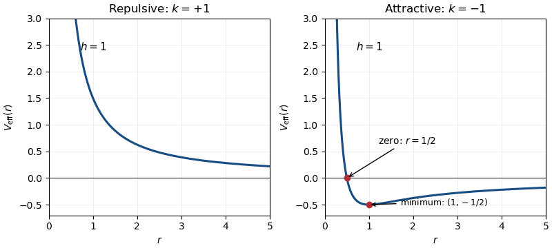
The given potential energy is $k/r$, whose radial force is $k/r^2$: positive $k$ is repulsive and negative $k$ attractive. The kinetic energy in polar coordinates is $({\dot{r}}^2+r^2{\dot{\theta }}^2)/2$, so conservation of energy givesFor $h\ne 0$ and $k>0$, the effective potential is positive, strictly decreasing from $+\infty$ to $0$, and has no stationary point. For $k=-\kappa <0$, it still tends to $+\infty$ at zero, crosses zero at $r=h^2/(2\kappa )$, and has its unique minimum atIt then approaches zero from below. The minimum corresponds to a stable circular orbit. If $h=0$, the centrifugal barrier disappears; the attractive effective potential is simply $-\kappa /r$ and has no minimum.

Interpret projection from very far away as the asymptotic incoming state at $r\to \infty$. For $v>0$ and impact parameter $b>0$, conservation of energy and conservation of angular momentum give $E=v^2/2$ and $|h|=bv$. At the closest approach the radial velocity vanishes. With $k=-\kappa <0$, the central-force radial turning point equation isOnly the positive root is physical. Put $q=\kappa /v^2$. The pericentre distance and the purely tangential speed there areThus $p<b$ and $u>v$: attraction bends the path inward and increases the speed. With positive energy, the Kepler orbit is a hyperbola. Measured from the pericentre direction, its polar coordinates satisfy $r=h^2/[\kappa (1+e\cos \varphi )]$ with $e=\sqrt{1+b^2{v}^4/{\kappa }^2}>1$.

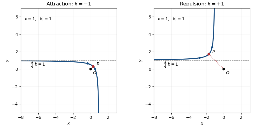
The hyperbola shown has a nonzero impact parameter. For $b=0$, the attractive radial orbit instead reaches the singular origin; there is no regular turning point with a finite closest-approach speed.

For $k=\kappa >0$, the same asymptotic data give $E=v^2/2$ and $|h|=bv$. At the central-force radial turning point,The positive root and the tangential speed, again with $q=\kappa /v^2$, areFor $b>0$, $\tilde{p}>b$ and $\tilde{u}<v$. The repulsive inverse-square force bends the trajectory away from the origin, as in the right-hand sketch. Its polar equation of a repulsive inverse-square orbit is $r=h^2/[\kappa (e\cos \varphi -1)]$, with $e=\sqrt{1+b^2{v}^4/{\kappa }^2}>1$ and $\varphi$ measured from closest approach.

For $b=0$, the regular radial turning point is $\tilde{p}=2\kappa /v^2$ and its speed is zero; the particle reverses direction there. The formula $bv/\tilde{p}$ still gives zero, while its rationalized form containing $1/b$ should be interpreted only by a limit.

For equal $|k|=\kappa$ in the two cases, their closest distances are conjugate roots expressed with the same $q=\kappa /v^2$. ConsequentlyAt either central-force radial turning point, the velocity is tangential and conservation of angular momentum gives $pu=\tilde{p}\tilde{u}=bv$. ThusThese attractive and repulsive inverse-square closest approaches pair a shorter, faster attractive passage with a longer, slower repulsive one. The speed-product conclusion assumes $b>0$; at $b=0$, the attractive orbit hits the singular centre with unbounded speed, so the formal product with the repulsive zero speed is not defined.

The rotating-frame derivative formula is $(d\mathbf{A}/dt{)}_S=(d\mathbf{A}/dt{)}_{S^{\prime }}+\mathbf{\omega }\times \mathbf{A}$. Applying it twice to the position vector, with constant angular velocity, givesSolving for ${\mathbf{a}}_{S^{\prime }}$ identifies the displayed terms: its left side is the acceleration relative to the rotating reference frame, the first right-hand term is the inertial acceleration, $-2\mathbf{\omega }\times {\mathbf{v}}_{S^{\prime }}$ is the Coriolis acceleration, and $-\mathbf{\omega }\times (\mathbf{\omega }\times \mathbf{r})$ is the outward centrifugal acceleration.

For a particle of mass $m$, replace ${\mathbf{a}}_S$ by the actual force divided by $m$ using Newton's second law. The remaining terms then appear as apparent forces in $S^{\prime }$. There is no Euler acceleration because $\mathbf{\omega }$ is constant and no translational acceleration term because the common origin is fixed in the inertial frame.

The original PDF measures $\theta$ at the rim point $O$, from the positive $x^{\prime }$-axis to $OP$; it is not the angle at the centre of the circle. The converted TeX omits this entire subpart. In rotating Cartesian coordinate system, the centre is $(a,0)$, and the nonzero intersection of the ray $\mathbf{r}=\rho (\cos \theta ,\sin \theta )$ with $(x^{\prime }-a{)}^2+y^{\prime 2}=a^2$ has $\rho =2a\cos \theta$. ThereforeThe second form stays regular even at the rim point $O$, where the polar radius is zero. Define the outward unit normal from the centre and the increasing-angle unit tangent vector byThe first two derivatives in the rotating reference frame are ${\mathbf{v}}^{\prime }=2a\dot{\theta }\mathbf{\tau }$ and ${\mathbf{a}}^{\prime }=2a\ddot{\theta }\mathbf{\tau }-4a{\dot{\theta }}^2\mathbf{n}$. These describe a bead on a horizontal hoop rotating about its rim.

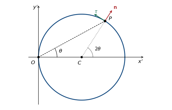
Because the contact is frictionless, the horizontal normal force is ${\mathbf{F}}_h=N\mathbf{n}$, with $N$ a signed outward component. Any vertical contact component balances Newtonian gravity and does not enter the horizontal equations. With $\mathbf{\omega }=\omega \hat{\mathbf{z}}$, the rotating reference frame equation givesSince $\hat{\mathbf{z}}\times \mathbf{\tau }=-\mathbf{n}$, $\mathbf{r}\cdot \mathbf{n}=2a{\cos }^2\theta$, and $\mathbf{r}\cdot \mathbf{\tau }=-a\sin 2\theta$, its normal and tangential components areHence the requested horizontal force vector isIts magnitude is the absolute value of the scalar coefficient. That coefficient need not always be negative: the constraint can exert either sign of normal force, depending on the bead's relative velocity. The tangential equation, which does not contain the reaction, is $\boxed{\ddot{\theta }=-({\omega }^2/2)\sin 2\theta }$.