Let and take without loss of generality. The Boussinesq approximation replaces density by in inertia and pressure acceleration, while retaining the density perturbation in buoyancy. Linearizing about the hydrostatic equilibrium and substituting the normal mode givesThe last two equations give and . The horizontal momentum equation givesSubstituting in the vertical momentum equation yields the Taylor–Goldstein equation:The buoyancy frequency is real for stable density stratification. The impermeable walls impose .
For a possibly unstable normal mode, ensures never vanishes, so choose one continuous branch of . Substitute into the Taylor–Goldstein equation and collect terms:Multiplication by puts its first two terms in divergence form:Multiply by the complex conjugate and apply integration by parts. Since , the boundary term vanishes and the power-transformed Taylor–Goldstein energy identity isThe weight is , not : preserving its complex phase is essential for the subsequent stability proofs.
Choose in the power-transformed Taylor–Goldstein energy identity and let . The result isBecause and , its imaginary part givesIf everywhere, the integral is strictly positive for every nonzero eigenfunction, so a mode with is impossible. Thus the flow is neutrally stable to these inviscid normal modes. This is the Miles–Howard theorem, expressed as a lower bound on the gradient Richardson number. It excludes exponential modal growth; it does not by itself exclude transient growth.
Choose . The power-transformed Taylor–Goldstein energy identity reduces toThe right side is real. For an unstable mode, , so taking the imaginary part givesConsequently the phase velocity is a weighted average:The weights are nonnegative and not identically zero. For a nonconstant shear profile, equality at an extremum would force to vanish on an interval where differs from that extremum; uniqueness for the regular ordinary differential equation would then give the zero mode. This is the phase-speed bound for unstable stratified shear modes.
Let be the displacement amplitude of an interface. Its kinematic boundary condition is , on either side, so the first of the jump conditions for stratified inviscid shear flow isFor zero surface tension, pressure is continuous at the displaced interface. Since the background hydrostatic pressure has derivative , linearization gives . Using and the kinematic condition givesThis derivation also works when jumps: the displacement is shared, while the vertical velocity need not be. It avoids ambiguous products of distributions at a discontinuous velocity profile.
Write , , and . The velocity is linear through all three layers, so and has no jump. Each interface has density drop . The jump conditions for stratified inviscid shear flow becomeBetween interfaces, the Taylor–Goldstein equation is . A decaying solution can therefore be writtenIts derivative jumps are , while its values at the interfaces are . Hence the coefficients satisfyThe determinant must vanish. With , and , one has . Expanding gives the dispersion relation for two density interfaces in uniform shear:
Put and . The dispersion relation for two density interfaces in uniform shear isIts discriminant is , so both roots are real. Their sum is positive; therefore one is negative precisely when their product is negative. That condition isSolving for givesIn this interval , so is the growing normal mode. At either endpoint the corresponding root is zero and the mode is neutral.
For large , the coupling is exponentially weak. If each interface were isolated, its interfacial gravity waves would have dimensional phase velocities , orThe upper-interface wave travelling against its positive local current has speed . The lower-interface wave travelling against its negative current has speed . Their laboratory speeds match at zero when . Weak interaction then produces counterpropagating wave instability rather than two independent travelling waves.
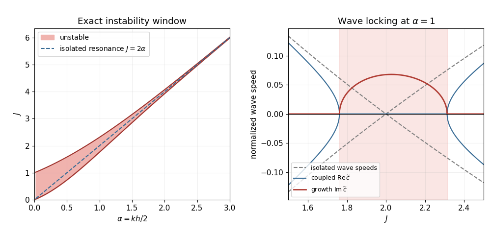

The band has the large-wavenumber form . Exactly at resonance, , soThus the instability window and growth rate both become exponentially small as the interfaces become weakly coupled.
For distinct eigenvalues, the formula holds for . If the lower-left entry of is , multiplication by gives . This proves by mathematical induction thatSumming the absolutely convergent matrix exponential series givesFor the repeated eigenvalue , the continuous limit is . This is also the exponential of a two-dimensional Jordan block.
Termwise differentiation of the matrix exponential gives and . Thus satisfies and the prescribed initial condition. Uniqueness for a linear differential equation makes it the solution.
For real , computeThus is a non-normal matrix. For distinct eigenvalues, takeThese satisfy but have inner product . The eigenvectors are therefore nonorthogonal. When the eigenvalues coincide, only the direction remains as an eigenvector; is a defective Jordan block.
Differentiate the quadratic energy:For , put . Immediate energy growth occurs precisely when . With both eigenvalues negative, such directions exist iff . Writing , the growing initial conditions are the two opposite open wedgesIf , energy decreases. No energy growth at any time, for any initial condition, is possible exactly whenIndeed, this makes the symmetric part of a matrix a negative semidefinite matrix, so along every trajectory. If the product is smaller, the wedges already supply counterexamples at . This is the instantaneous energy-growth criterion for a linear system.
At each fixed time, the maximum over nonzero initial conditions is the optimal energy amplification of a linear system:Write , and . The symmetric matrix has trace and determinant . Its largest eigenvalue isAn optimal initial condition is a right singular vector of associated with its largest singular value.
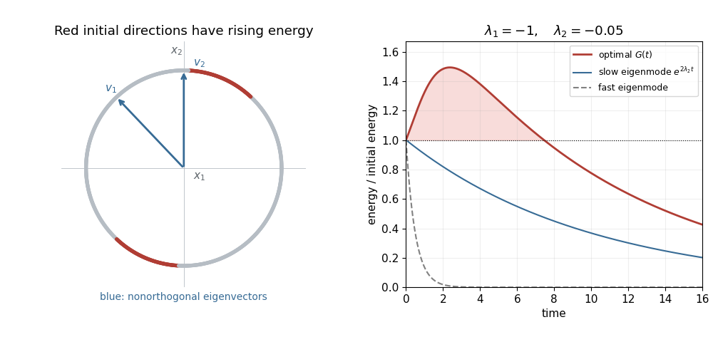
Stable eigenmodes can combine to produce transient energy growth
. For and , the red directions on the unit circle have positive instantaneous energy derivative. The eigenvectors are nonorthogonal. The right panel compares the optimal energy amplification of a linear system with the monotonically decaying energy of each eigenmode. Details.
If , let . Then , so the precise long-time asymptotic statement isThe Cauchy-Schwarz inequality shows that the unit initial conditions achieving this leading factor areThis is an adjoint eigenvector, since . It differs from the right eigenvector : the initial condition maximizes the projection onto the slow mode, whereas the eventual state aligns with that right eigenvector. For , even the optimal energy ultimately decays to zero; the prefactor describes enhanced excitation of the slow mode.
The zero streamfunction gives zero velocity. The temperature obeys both prescribed temperature values, has no horizontal gradient, and has zero Laplacian. Thus it satisfies both equations with :This is the conductive state of Darcy-Bénard convection.
Linearizing about the conductive state givesThe perturbations vanish at . For a normal mode with vertical dependence , put . The two modal equations are and . Eliminating givesNeutrality requires . The arithmetic-geometric mean inequality bounds this below by , with equality at . The first unstable vertical mode is therefore , givingThe wavelength statement applies at the first onset. At a general larger , maximizing the growth rate within a fixed vertical mode gives , so its preferred wavelength need not remain exactly two. This is the onset of convection in a horizontal Darcy layer.
The full perturbation equations arewhere the streamfunction advection bracket is . Put and introduce the slow time , so on the amplitude-dependent fields. ThenThe weakly nonlinear expansion balances the small linear growth against the cubic saturation on this slow time scale.
At first order, and . Since and , the first equation fixes . The homogeneous temperature boundary conditions and the second equation remove any horizontally uniform term, givingAt second order,The forcing is horizontally uniform. Taking no additional critical-mode component, a solution satisfying the homogeneous boundaries isThis mean-temperature correction in weakly nonlinear Darcy convection modifies the vertical temperature gradient and provides the feedback that saturates the convection.
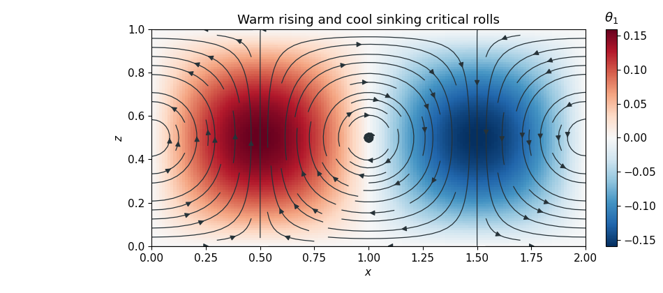

Let and denote the full third-order coefficients. This notation keeps the detuning term, proportional to , and the slow-time term, proportional to , visible. DefineThe equations at order areEquivalently, where , the question's coefficients satisfy and . Eliminate from the full coefficients:Use the Fredholm solvability condition for a self-adjoint operator. With , projection onto the critical eigenfunction makes the left side vanish. Therefore the Landau amplitude equation isThese integrals already answer the requested coefficient calculation. Evaluating them gives , , and . Hence, for the prescribed normalization,The cubic term opposes growth, so the nonzero steady amplitudes are stable equilibria within the chosen roll phase. The conductive state is unstable for this positive detuning. This is supercritical saturation of Darcy convection rolls.
Articles by others on the same topic
There are currently no matching articles.