Past exam of the physics course of the year 4 of the natural sciences course of the University of Cambridge / 2012 / Paper 1 / Section B

A normal mode is a small motion in which all coordinates oscillate at one common angular frequency with fixed relative amplitudes. For conservative linearized motion, these are eigenvectors of the mass-weighted stiffness matrix.

All three springs are initially stretched from $l$ to $2l$, giving equal tension $T_0=kl$ and zero resultant force on each mass. This prestress is essential for the transverse modes found below.

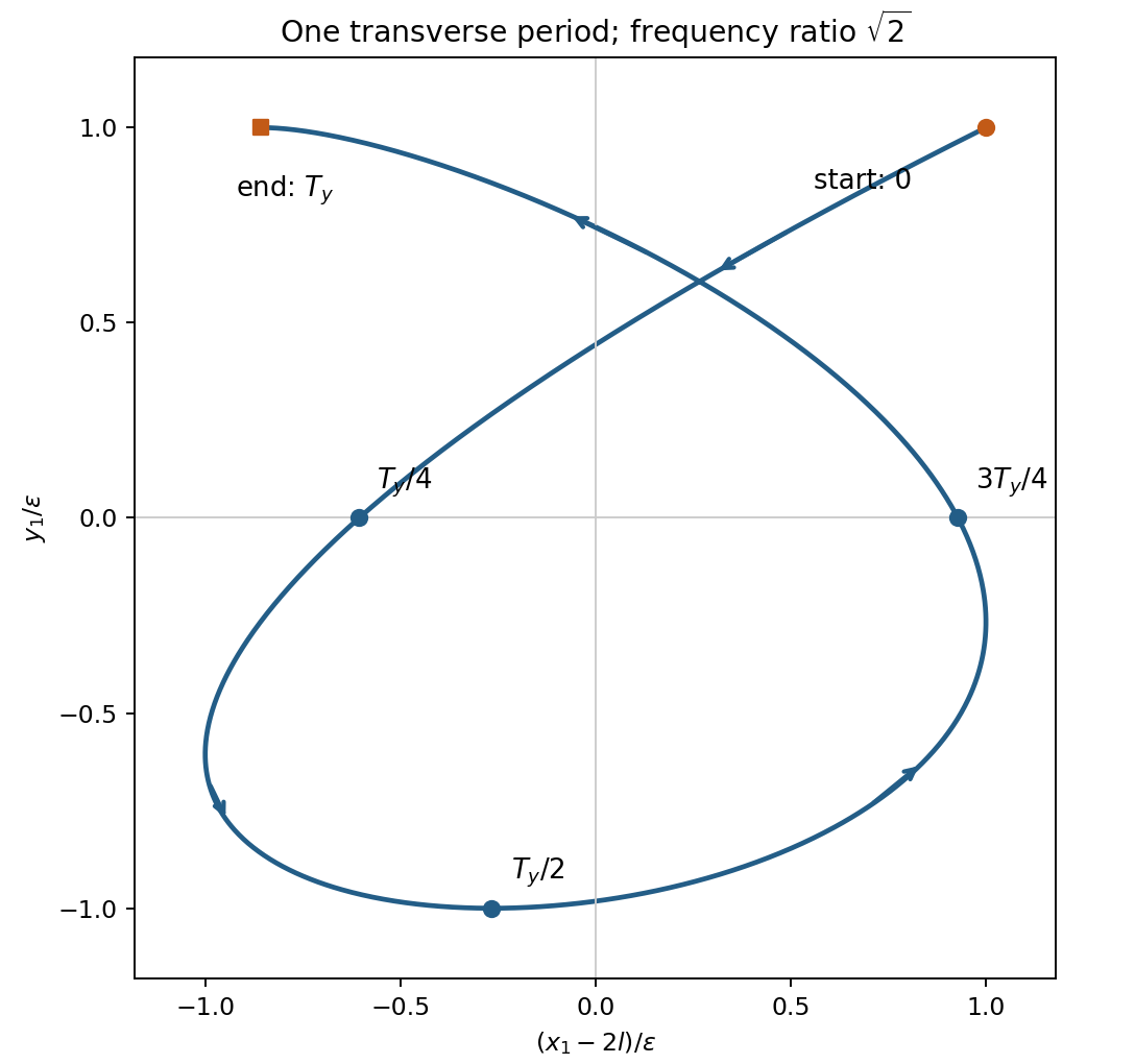
For the final mixed-axis trajectory of a prestressed spring pair, the initial displacements excite only the symmetric mode in each direction. Therefore, to first order in $ϵ/l$,The second mass has the same displacements about $4l$. Over the first transverse period $T_y=2\pi \sqrt{2m/k}$, write $s=t/T_y$:The trajectory is not closed after $T_y$, because the frequency ratio is $\sqrt{2}$. It ends at approximately $(-0.858,1)$ in these scaled coordinates rather than $(1,1)$.

Let $X_1,X_2$ be longitudinal displacements. Hooke's law givesThe symmetric and antisymmetric eigenvectors are respectively $(1,1)$ and $(1,-1)$, soOrdinary frequencies are these values divided by $2\pi$.

The transverse stiffness of a stretched spring follows because a spring of length $2l$ develops transverse force $T_0\Delta y/(2l)$ to first order. Its extension changes only at second order, so the leading transverse stiffness comes from its existing tension, not from that extension change. Here $T_0/(2l)=k/2$, givingThe mode vectors are again $(1,1)$ and $(1,-1)$. Treating the springs as unstretched would incorrectly remove this linear restoring force.

The first-order grating equation is $d\sin \theta =\lambda$, so $d=2.879\mu \mathrm{m}$, about $347$ lines per millimetre. For $N$ equally illuminated lines,Principal maxima stay at the same angles, their peaks scale as $N^2$ for fixed illumination per line, and their angular widths shrink as $1/N$. The resolving power of a diffraction grating is $\lambda /\Delta \lambda =mN$. Thus first order needs $N=1000$ and illuminated width $Nd\simeq 2.88\mathrm{mm}$.

The grating dispersion follows by differentiation: $d\theta /d\lambda =1/(d\cos \theta )$. With a detector centred on the chief ray, one pixel corresponds approximately toThis exceeds the nominal $0.5\mathrm{nm}$ grating width. The practical resolution scale is therefore a few nanometres; two-pixel sampling gives about $4.5\mathrm{nm}$. Exact resolvability also depends on slit width and image sampling. Taking the detector coordinate as $f\tan \theta$ about the original axis instead changes the single-pixel estimate only to $2.20\mathrm{nm}$.

For ideal photon counting, Poisson distribution statistics give SNR $=\sqrt{N_{\gamma }}$. Hence $N_{\gamma }=10^4$ and $t_{\min }=10^4/(2\times 10^5)=0.050\mathrm{s}$.

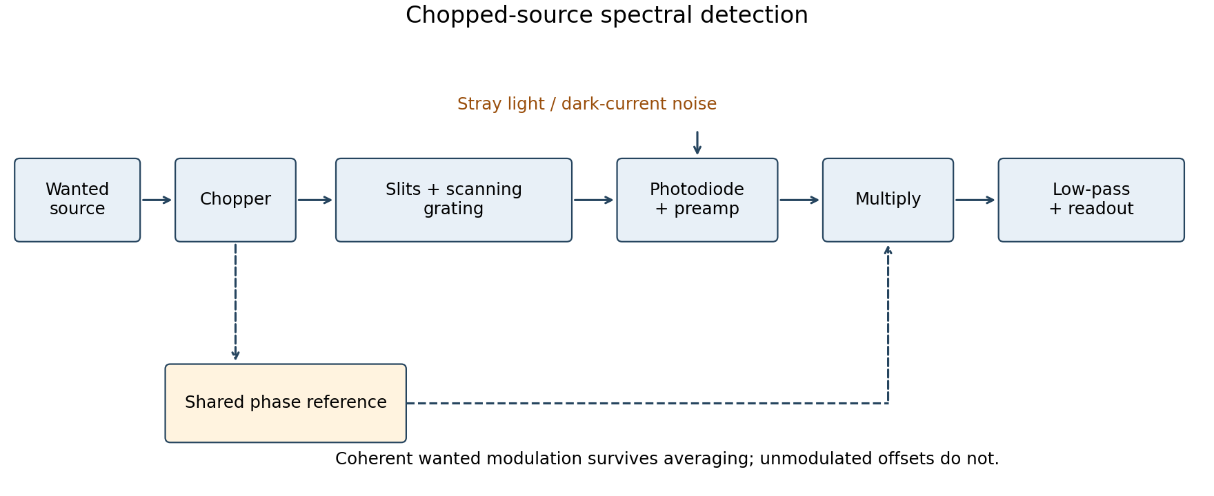
Use a lock-in amplifier for phase-sensitive detection: chop or otherwise modulate the source before the entrance slit, retaining a synchronous reference. At each grating setting amplify the photodiode output, multiply it by a reference and low-pass filter. For a signal $s\cos ({\omega }_{r}t+\varphi )$ and reference $2\cos {\omega }_{r}t$, the low-pass output is $s\cos \varphi$; quadrature demodulation also recovers $s\sin \varphi$. Choose the modulation frequency above slow drift while within the source/detector bandwidth and away from strong electrical interference. Average for many cycles before changing the grating setting.

This rejects steady backgrounds and reduces low-frequency noise through narrow-band detection. It does not remove random dark-current/stray-light shot noise within that bandwidth, nor a background modulated coherently with the source. The chopping geometry must therefore distinguish wanted light from stray paths.^[ref]

With microstate energies held fixed when differentiating,Since $d\beta /dT=-1/(k_B{T}^2)$,The canonical ensemble fixes volume and particle number, and any other external Hamiltonian parameters. Thus the derivative is $C_V$; pressure-fixed fluctuations would naturally involve enthalpy in a different ensemble.

The translational and two-level energy variance follows because translation and internal states factorize for this dilute classical gas:Differentiating twice yieldsThe terms are independent translational and two-level binomial variances. At $k_{B}T\ll ϵ$, excitation freezes out exponentially and translation dominates. At $k_{B}T\gg ϵ$, the internal variance tends to $N{ϵ}^2/4$ while the translational variance grows as $T^2$; the internal heat capacity consequently tends to zero. Fractional total-energy fluctuations are of order $N^{-1/2}$ for large $N$. The low-temperature statement presumes translation is still nondegenerate; at strictly zero temperature the classical-gas model fails.

Use energy units $m=m_p{c}^2$, $M=m_A{c}^2$, $e=E_{\gamma }$ and $P=pc=\sqrt{E^2-m^2}$. The soft-photon resonant capture threshold follows from four-momentum conservation:For fixed proton energy the left side is largest at head-on incidence. Its threshold is $E+P=2E_0$. Combining that with $(E-P)(E+P)=m^2$ givesEquality is allowed for a head-on photon. Here $e=k_{B}T=2.3482\times 10^{-4}\mathrm{eV}$, soA very soft photon needs an enormous proton Lorentz factor to reach the specified invariant mass. A true thermal photon distribution and a finite-width resonance would smear this monoenergetic threshold.

For $\theta =0$, $E-P=m^2/(E+P)\le m$, whereas $2E_0\gg m$, so production is impossible. For each nonzero angle, sufficiently large energy is possible, and $P\simeq E$ givesTo find the maximum deflection in soft-photon capture, note that the final particle's transverse momentum comes entirely from the photon:Writing $x=\cos \theta$, maximization gives $(1-x)(2x+1)=0$ and the interior maximum $x=-1/2$. Therefore, to the same extraordinarily accurate ultrarelativistic order,The neglected relative corrections are of order $m^2/E_0^2$ and $e/E_0$, both around $10^{-24}$. The final particle is effectively collinear with the proton despite a large photon incidence angle.

In the weak-field Zeeman effect, spin-orbit coupling keeps $L,S,J$ good and a level shifts by ${\mu }_B{g}_{J}B{m}_J$. At fields large compared with fine-structure coupling but still within the linear electronic Zeeman approximation, $L$ and $S$ decouple: the Paschen-Back effect gives shifts ${\mu }_{B}B(m_L+2m_S)$. Electric-dipole transitions obey $\Delta m_L=0,\pm 1$, $\Delta m_S=0$ in that limit, recovering an orbital triplet pattern. Intermediate fields mix the coupled states.

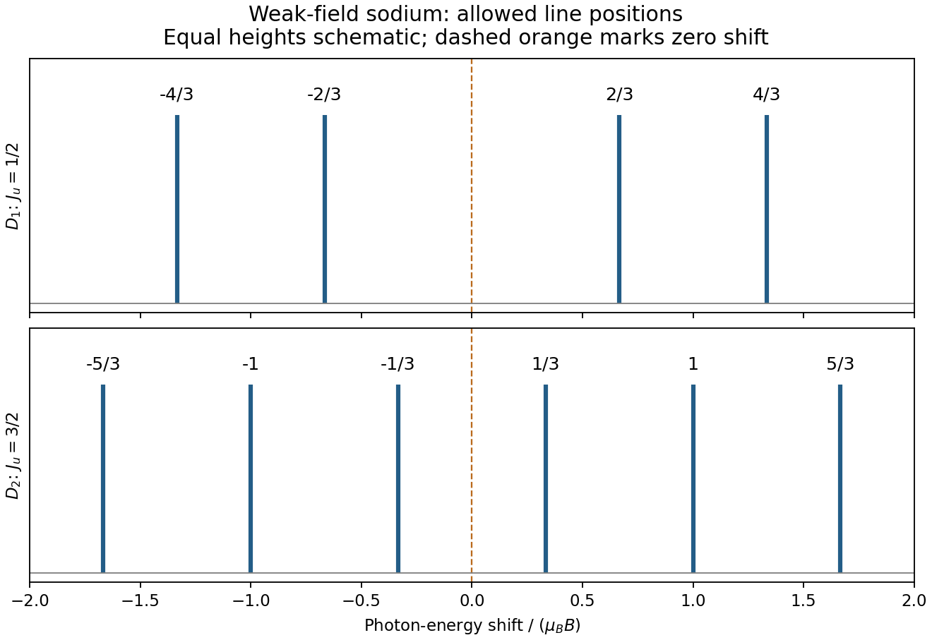
For the weak-field sodium D-line Zeeman pattern, the given Landé g-factor formula givesAllowed photon shifts are $\delta E={\mu }_{B}B(g_u{m}_u-2m_l)$ with $m_u-m_l=0,\pm 1$. ThusThese are the four- and six-component patterns. Both $\pi$ and $\sigma$ components are represented, so an observation strictly along the field, which removes $\pi$ emission, would not show this complete pattern. Hyperfine structure is neglected.

To determine the magnetic field from a Zeeman diagram, the unsplit separation provides its energy scale:The smallest adjacent split spacing $s_E=2{\mu }_B{B}_1/3$ is approximately $0.070$ of that separation in the sketch. ThereforeThis is a graphical estimate; the drawing does not warrant high precision. Its splitting energy is small compared with $\Delta E_D$, consistent with the weak-field approximation.

For Doppler resolution of a Zeeman pattern, thermal velocities give Gaussian Doppler broadening with widthAt $350\mathrm{K}$, the photon-energy FWHM near $589\mathrm{nm}$ is $5.88\times 10^{-6}\mathrm{eV}$. Equating the smallest adjacent Zeeman spacing to this width gives $B\sim 0.15\mathrm{T}$ for loss of individually resolved components. There is no sharp Gaussian resolution threshold; using whole-pattern width instead gives a smaller field of order $0.03$–$0.04\mathrm{T}$ for complete disappearance into a single envelope. Instrumental and collisional broadening would also affect the estimate.

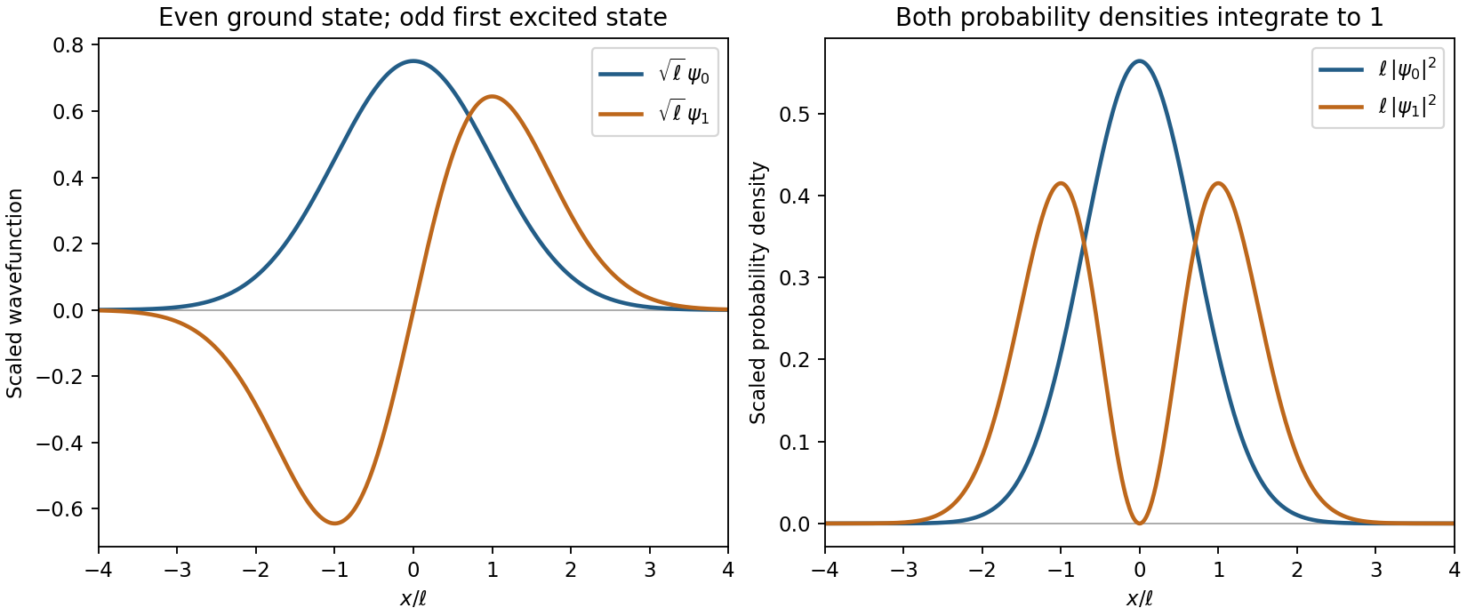
For the quantum harmonic oscillator, using $[\hat{x},\hat{p}]=i\hslash$, direct multiplication givesThe commutators areThus each ladder operation shifts energy by one quantum. The ladder operator norms $\Vert a|n⟩{\Vert }^2=n$ and $\Vert a^{†}|n⟩{\Vert }^2=n+1$, with conventional phases, giveLet $\ell =\sqrt{\hslash /(m\omega )}$. In position space $\hat{p}=-i\hslash {\partial }_x$, so $a{\psi }_0=0$ becomes $(x+{\ell }^2{\partial }_x){\psi }_0=0$. Normalizing and then applying $a^{†}$ givesTheir overlap vanishes because ${\psi }_0^{\ast }{\psi }_1$ is odd on the full real line; the Gaussian second moment verifies $\int |{\psi }_1{|}^{2}dx=1$.

For a normal from medium 1 to 2, the magnetic boundary conditions areWithout a free surface current, tangential $H$ is continuous. To obtain the magnetization of a permeable sphere of radius $R$ and permeability ${\mu }_0(1+\chi )$, choose magnetic scalar potentialsTangential continuity gives $H_i=H_0-C/R^3$, and normal $B$ continuity gives $(1+\chi )H_i=H_0+2C/R^3$. HenceThe fields are uniform inside. For negative susceptibility, magnetization is antiparallel to the applied field; the scalar formula retains its negative sign.

For a small weakly magnetic body, the induced magnetic energy is $U_m=-\chi V{B}^2/(2{\mu }_0)$. The factor one-half accounts for building the induced moment. The vertical force is $F_z=\chi VB{B}^{\prime }/{\mu }_0$. Balancing gravity therefore givesA diamagnet needs a field decreasing in magnitude with height for an upward force. For diamagnetic levitation in an inverse-height field,The force falls as $z^{-3}$, giving a restoring vertical derivative at equilibrium. Full lateral stability would require the transverse field geometry, which is not specified.

The far fields obey $E_{\theta }=c{B}_{\varphi }$. The radial component of their Poynting vector is $E_{\theta }{B}_{\varphi }/{\mu }_0$. Averaging ${\ddot{p}}^2=p_0^2{\omega }^4{\cos }^2\omega (t-r/c)$ and integrating $\int {\sin }^2\theta d\Omega =8\pi /3$ givesFor a small isotropically polarizable particle, $p_0=\alpha E_0$ and incident intensity is $I={ϵ}_{0}c{E}_0^2/2$. Thus the total Rayleigh scattering cross-section isEach incident linear polarization gives the same integrated power; averaging unpolarized light does not add another factor of two. The scalar real polarizability approximation neglects absorption and molecular anisotropy.

For Rayleigh attenuation from refractivity in dilute air, polarization density is $\mathbf{P}=N\alpha \mathbf{E}$. Consequently ${ϵ}_r=1+N\alpha /{ϵ}_0$ and, with ${\mu }_r\simeq 1$ and $n-1\ll 1$,The ideal-gas number density at the supplied pressure and temperature is $N=P/(k_{B}T)=2.47\times 10^{25}{\mathrm{m}}^{-3}$, yielding $\alpha =2.15\times 10^{-40}\mathrm{C}{\mathrm{m}}^2{\mathrm{V}}^{-1}$. For an explicit representative visible wavelength $\lambda =550\mathrm{nm}$,Direct-beam intensity follows $I(x)=I(0)e^{-x/L_{\mathrm{att}}}$. Equivalently $L_{\mathrm{att}}=3N{\lambda }^4/[32{\pi }^3(n-1{)}^2]$. Its strong wavelength dependence gives roughly $21$–$200\mathrm{km}$ across $400$–$700\mathrm{nm}$ if refractivity is held fixed. This is a uniform-density dry-air scattering estimate, not absorption or transmission through a vertically stratified atmosphere; aerosols and molecular depolarization corrections are outside the given model.