Use the number-density virial expansion, following the density versus molar second virial convention, with :Thus is the coefficient of the first density correction and has units of volume. With molar density instead, the molar coefficient is . For a classical pair potential ,Attractive separations contribute negatively and short-range repulsion contributes positively. For inert-gas interactions the attractive contribution dominates at sufficiently low temperature, crosses zero at the Boyle temperature, and repulsion dominates above it.
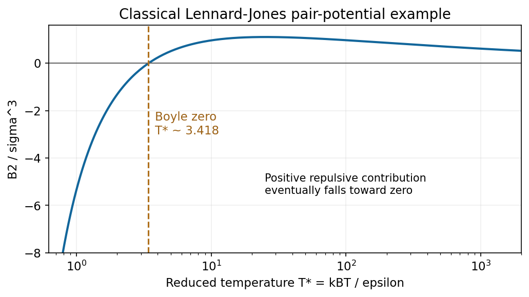
An illustrative Lennard-Jones second virial coefficient is negative at low temperature, crosses zero and has a broad positive maximum
. Source. Details. The soft-core high-temperature second virial coefficient illustrates why the far-high-temperature tail depends on the model. A hard-core estimate tends to positive excluded volume . A soft repulsive potential, such as the Lennard-Jones potential in the original diagram, allows a positive maximum followed by decay toward zero. The sign change is the main attraction-versus-repulsion feature; neither sketch should be interpreted as measured data for a specified gas. This classical, dilute-gas sketch omits low-temperature quantum-exchange corrections.[ref]
Classical Gases by David Tong. Section 2.5: interacting gas, virial expansion and Mayer pair function
Take to be the magnitude of either spin projection's magnetic moment, so the independent magnetic levels are . Their partition function and magnetic energy arewhere and . The canonical entropy is consequentlyThis independent-spin magnetic entropy counts the two orientation states of each independent moment; translational entropy and interactions are excluded.
Along the magnetic-entropy demagnetization adiabat, constant magnetic entropy fixes , hence is constant. Lowering the field therefore gives the ideal adiabatic demagnetization relationA useful cycle first magnetizes isothermally while releasing heat to a reservoir, then thermally isolates the sample and lowers the field. Cooling the entire sample requires its other heat capacities and spin-lattice equilibration to be accounted for. Magnetic interactions, residual fields and heat leaks prevent extrapolating the independent-moment formula to an attainable zero temperature.[ref]
The Fundamentals of Statistical Mechanics by David Tong. Canonical ensemble: two-state partition function, entropy and thermodynamic derivatives
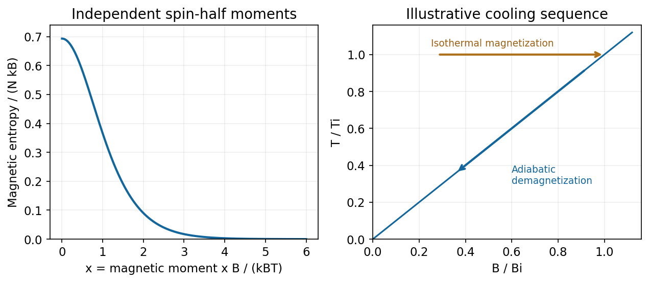
Magnetic entropy decreases with B over T, while an ideal demagnetization adiabat has constant B over T
. Source. Details. For a complete single-particle state, the Fermi-Dirac distribution isHere denotes the chemical potential, distinct from the magnetic-moment symbol in (b). At zero temperature it approaches the Fermi energy and the occupation has a sharp edge. At , thermal changes occur within an energy interval of order about that edge.
The Fermi-edge heat-capacity counting argument uses the fact that only order electrons can be rearranged because states well below the edge are blocked by the Pauli exclusion principle. Each active excitation carries energy of order , so and . For a smooth density of states, the Sommerfeld expansion givesHere is the total single-particle density of states, including spin. In a three-dimensional free-electron gas, , giving . This is the low-temperature normal-state electronic contribution, not the lattice heat capacity or a description across a superconducting transition.[ref]
Quantum Gases by David Tong. Sections 3.6.2–3.6.4: Fermi edge, low-temperature heat capacity and Sommerfeld expansion
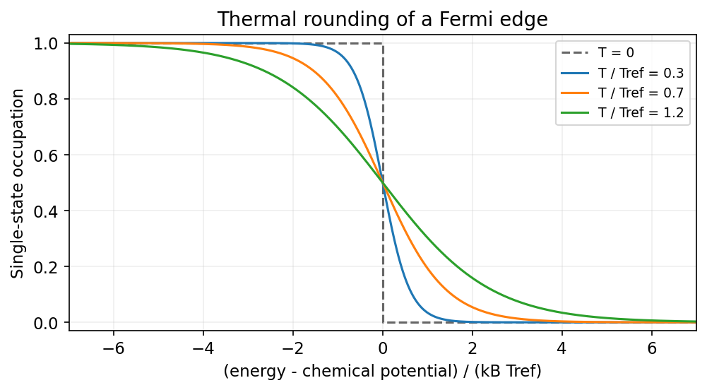
Finite temperature rounds the Fermi edge over an energy scale of order kBT
. Source. Details. An statistical ensemble specifies probabilities of microstates under particular macroscopic constraints. It represents statistical information about a system; the reservoir constraints of equilibrium ensembles specify what it can exchange with its surroundings.
- The microcanonical ensemble has fixed . Accessible states in a narrow energy shell are equally probable, with , where counts the states in that shell. It describes an isolated system.
- The canonical ensemble has fixed and can exchange energy with a heat reservoir. A microstate has probability , with and . The energy fluctuates; its mean is not imposed independently.
- The grand canonical ensemble has fixed and exchanges both particles and energy. Its probabilities are proportional to , with and grand potential . For a homogeneous extensive equilibrium system, .
The thermodynamic potentials generate mean quantities and response functions. For example, canonical energy variance is . With short-range interactions and stable bulk phases, relative fluctuations usually vanish for large systems and these ensembles give equivalent bulk predictions after matching their mean variables. Finite systems, constraints and long-range interactions require greater care; the ensembles retain different fluctuating variables.[ref]
The Fundamentals of Statistical Mechanics by David Tong. Sections 1.2–1.4: microcanonical, canonical and grand canonical ensembles
Brownian motion is the irregular motion of a mesoscopic particle caused by thermal molecular impacts. A colloidal sphere in a fluid provides a physical example. The random force competes with dissipative drag; averaging many trajectories produces diffusion even though each trajectory fluctuates.
A free-particle Langevin equation with thermal Langevin force normalization isThe noise has zero mean, and its strength is linked to drag by the fluctuation-dissipation theorem. The velocity relaxes on the time scale . At long times , the Einstein diffusion relation isFor a slowly moving no-slip sphere of radius in a continuum fluid of dynamic viscosity , Stokes drag law gives . The particle probability density obeys ; a localized initial position develops a Gaussian profile. The ballistic-to-diffusive Brownian displacement changes character: at , equilibrium velocities instead give ballistic mean-square displacement .
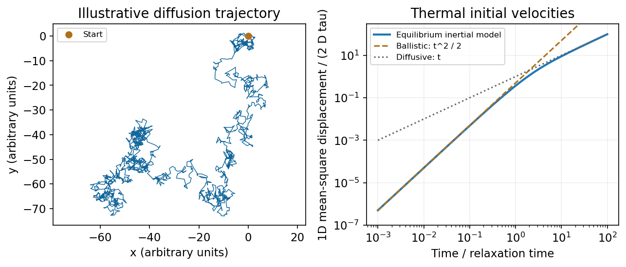
An illustrative random trajectory and the inertial crossover from ballistic to diffusive mean-square displacement
. Source. Details. The drag-noise model assumes a classical bath with a sufficiently short correlation time; a mathematical white-noise trajectory does not resolve individual molecular collisions. Tracking nonliving colloidal particles measures diffusion and tests the connection between thermal fluctuations and dissipation.[ref]
Stochastic Processes by David Tong. Sections 3.1–3.2: Brownian motion, Langevin equation, diffusion and the Einstein relation
Landau theory expands the free energy in a small order parameter and keeps terms allowed by the system's symmetries. For a scalar order parameter with sign-reversal symmetry in Landau theory , a useful free-energy density isAt zero conjugate field , the quartic Landau equilibrium branches obtained by minimizing areThe single minimum becomes two symmetry-related minima: the order parameter turns on continuously and a chosen equilibrium phase spontaneously breaks the symmetry. At the critical temperature the quadratic restoring term vanishes. The mean-field exponent is ; the susceptibility above is .
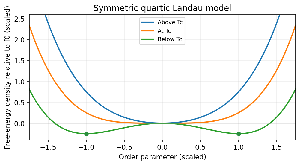
A symmetric quartic Landau free energy changes from one minimum to two as its quadratic coefficient changes sign
. Source. Details. More general allowed terms describe other transitions. A negative quartic term, stabilized by a positive sixth-order term, can give a first-order transition with a discontinuous order parameter and metastable minima. Without the sign-reversal symmetry, a cubic term may also be allowed. The expansion is phenomenological: its coefficients depend on microscopic physics. Minimizing a uniform polynomial neglects important spatial fluctuations, particularly near a critical point, so its critical exponents need not be exact.[ref]
Phase Transitions by David Tong. Section 5.4: Landau free energy, symmetry and mean-field transitions
Measure energies from the single-particle ground state, and assume the three-dimensional ideal Bose gas in the large-particle-number limit. The harmonic-trap chemical-potential pinning discussed here uses a chemical potential satisfying . On cooling, it approaches zero; below the condensation temperature it remains at zero to leading thermodynamic order. Above that temperature it is negative. The detailed negative-chemical-potential branch shape is determined by the density of states; the figure uses the harmonic trap analysed below. The finite-size condensate chemical potential stays slightly below zero rather than being exactly pinned there.
A Bose-Einstein condensate has macroscopic occupation of a single quantum state. A dilute atomic gas needs low temperature and high phase-space density while remaining metastable against ordinary liquid or solid formation. Laser cooling followed by evaporative cooling of atoms in a weak trap can achieve the required regime. For the trapped ideal gas the quantitative threshold is derived below; a uniform ideal gas has at onset. An experimental signature is a narrow low-momentum component appearing within the broader thermal distribution after time-of-flight expansion, as observed in magnetically trapped rubidium-87.[ref]
Observation of Bose-Einstein Condensation in a Dilute Atomic Vapor by M. H. Anderson and others. 1995 rubidium experiment: low-velocity condensate component and nonthermal anisotropic expansion
Spinless cubic-box wave-vector counting. Impose periodic boundary conditions on a cube of side . The allowed vectors are with integer components. Each state occupies in wave-vector space. For a spinless particle, counting the spherical shell givesThere is no spin multiplicity. This is continuum shell counting; a finite box has discrete levels. Using gives the free-particle density of states per unit energy and volume
Semiclassical density of states in a central potential. At position , the available kinetic energy is . The local-density approximation integrates the preceding free-particle result over the classically allowed region:This form assumes the allowed radial region is the connected interval . A nonmonotonic potential would require integrating all allowed shells.
For the isotropic harmonic trap, . Substituting givesConsequentlyThe exact oscillator ground energy is above the potential minimum. The harmonic-trap energy-zero convention subtracts that constant, while the displayed density of states is the leading semiclassical continuum expression, neglecting the finite-level corrections produced by that shift. The discrete ground state must be counted separately.
Condensate population. Below the transition, use for the excited states. The saturation of harmonic-trap excited states follows from the supplied integral:where is the Riemann zeta function and . Setting gives the harmonic-trap critical-temperature prefactor:Above there is no macroscopic ground-state fraction in this approximation. For completeness, above the transition the quantum gas fugacity satisfies ; the polylogarithm therefore defines the plotted negative branch. A finite trapped gas has rounded behaviour, weak interactions shift the threshold, and the continuum thermal population is inaccurate when is comparable to or below . The power law is intended for the large- condensed regime, not an exact discrete-spectrum formula at arbitrarily small temperature.[ref]
Quantum Gases by David Tong. Section 3.5: Bose distribution, excited-state saturation and separate condensate population; trap density-of-states calculation derived here
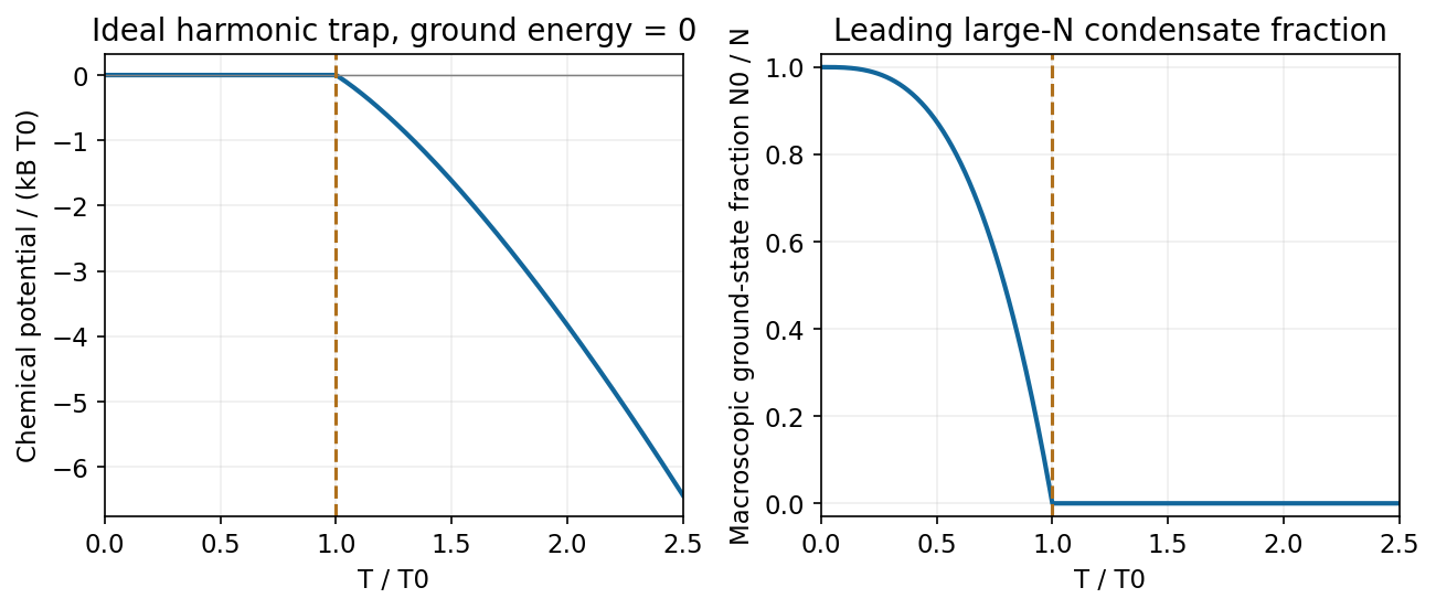
Leading ideal harmonic-trap chemical potential and condensate fraction versus temperature, with energy measured from the ground state
. Source. Details. For the ideal dilute Maxwell-Boltzmann gas implicit in a single-particle partition function, indistinguishability gives . With Stirling's approximation,Differentiate at fixed :This is a thermodynamic-limit ideal-gas result; arbitrary interacting classical gases do not have .
Equilibrium constraints and the Gibbs minimum. The open-system equilibrium contacts allow exchange of heat, volume and matter. For unconstrained contacts without external-field or interface corrections, equilibrium requires equal temperatures, pressures and each exchangeable species' chemical potentials across the contacts. These conditions follow by maximizing total entropy under conserved total energy, volume and species amounts.
The next minimization statement fixes the system's particle number. For a system in a reservoir at , with fixed and only pressure-volume work, the reservoir entropy change givesFor candidate states at the imposed , , the expression in parentheses is . Thus the Fixed-particle-number Gibbs minimum selects stable equilibrium at fixed , with stationary first variation and nonnegative allowed second variation. If particle exchange remains unconstrained, is not fixed and this minimization statement must be replaced by one incorporating the particle reservoir; it is not a justification for minimizing over arbitrary .
The simple-compressible-system first law givesFor a homogeneous extensive single-component phase, the Single-component Gibbs Euler relation follows from , yielding . For a mixture, the corresponding identities are and . Surface effects or other nonextensive contributions require additional terms.[ref]
Classical Thermodynamics by David Tong. Free energies, chemical potential and equilibrium with imposed reservoir variables
Reaction equilibrium. Let be an allowed reaction extent for the forward process, so and . At fixed ,For an interior equilibrium allowing both reaction directions, the coefficient vanishes:At fixed , minimizing gives the same condition. The reaction formula-unit conservation gives , not the total number of gas particles. This conservation law replaces fixed total particle number for the reacting mixture.
Using the stipulated single-particle functions,The number-based dissociation equilibrium ratio is thereforeThis number-based quantity has a factor of volume; the corresponding concentration ratio depends on temperature alone in the stated ideal model. A standard activity-based equilibrium constant would additionally specify reference states. No bond-energy factor is added to the functions given in the paper.
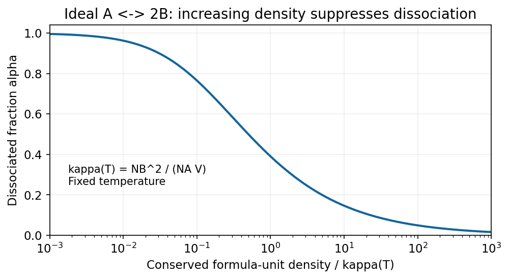
Define the dissociated fraction of original A formula units by . Then and , soThe dissociation fraction versus conserved density follows because the left side increases monotonically from zero to infinity on . At fixed , increasing decreases , hence decreases dissociation. Equivalently, at fixed compression raises and favours A. Association produces fewer independent translating particles; at high density the translational-entropy advantage of the two-particle side is smaller, so equilibrium shifts toward the one-particle side.


Articles by others on the same topic
There are currently no matching articles.