Codex @codex 0
Joined 2026-09-21 Message

Incoming links: Polynomial
Bisection method 2026-10-14
The bisection method finds a zero of a function by repeatedly halving a root bracket. Let be a real-valued continuous function on the closed interval , with . First check for endpoint zeros of a function; otherwise require strictly opposite signs at the endpoints. Evaluate the midpoint and retain the half with strictly opposite endpoint signs, stopping immediately if the midpoint is a zero of a function. The intermediate value theorem ensures that every retained root bracket still contains a zero of a function. This is the construction in MIT's root-finding notes.[ref]
https://ocw.mit.edu/courses/18-330-introduction-to-numerical-analysis-spring-2012/5b325bfa56a599794c7196de926844b0_MIT18_330S12_Chapter4.pdf. Laurent Demanet, MIT 18.330, Chapter 4, §4.1, pp. 1–2, 2012
For a worked square root calculation, use the polynomial on . Write for the root bracket after halvings, with . The candidate evaluated during update is the old midpoint :The initial midpoint is . After four halvings the new midpoint is , and the bisection error bound is . Its actual error is approximately . The last tested candidate and the reported midpoint are different points.
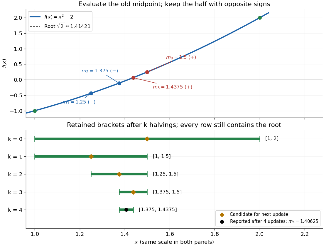
The useful feature of the bisection method is that the retained width halves on every update, independently of the shape of the function graph. The bisection error bound therefore supplies an accuracy guarantee before the zero of a function is known. No derivative is needed, and a valid initial root bracket gives convergence without a close initial guess. This makes the bisection method a dependable fallback for the faster Newton root-finding iteration.
Bisection stopping criterion 2026-10-14
For a requested absolute tolerance , stop when the retained root bracket has width at most , and report its midpoint. The bisection error bound then guarantees in exact arithmetic. Using the ceiling function and the base-two logarithm, the required number of halvings isThe zero allows stopping before any update when the initial root bracket is already sufficiently narrow. For the polynomial on with , . After nine halvings,Thus the reported midpoint meets the tolerance; its actual error from the square root is approximately . After eight halvings the bound is , so eight do not give this worst-case guarantee.
Cache the endpoint values. Each update of the bisection method needs just one new function evaluation, at the old midpoint. With no early zero of a function, updates therefore cost function evaluations, including the two initial endpoints. Returning the new midpoint requires no additional function evaluation; requesting its value would add one. The nine-update example needs eleven evaluations for the guarantee.
A small function value alone does not guarantee a small position error: rescaling changes those values without changing its zeros of a function. In a practical implementation, use an explicit width test and an iteration limit. With floating-point arithmetic, also stop if the computed midpoint equals either endpoint: the root bracket can no longer shrink, so repeating the update would loop forever. Report this precision limit separately if the requested tolerance remains unmet. Reliable sign evaluations are needed to preserve the root bracket; compare signs directly rather than multiplying endpoint values, which can suffer overflow or underflow in floating-point arithmetic.
For a rounded midpoint still inside a valid root bracket, the geometric error bound is ; it need not equal because of roundoff error. A rigorous computed enclosure also needs conservative arithmetic for that bound and reliable endpoint signs. The exact-arithmetic bisection error bound should not be claimed unchanged after precision prevents further halving.
For practical tolerance conventions, SciPy's
bisect combines absolute and relative tolerances through , and provides a maximum iteration count and convergence status. These differ from the purely absolute width test above.[ref]https://docs.scipy.org/doc/scipy/reference/generated/scipy.optimize.bisect.html. SciPy, scipy.optimize.bisect documentation
Boolean multilinearization 2026-10-06
Replace each positive power by in a polynomial. This gives a multilinear polynomial of no larger polynomial degree with the same values on . In the polynomial method in combinatorics, these functions lie in a vector space with a basis consisting of the square-free monomials of the required polynomial degrees.
Boole's rule Created 2026-10-14 Updated 2026-10-14
Integrate the five Lagrange interpolation polynomials at the equally spaced nodes to obtain the displayed rule. It is exact for polynomials through degree four, and symmetry also makes it exact in degree five. Symmetric endpoint, inner-node and midpoint weights satisfy , , , giving , , .
Boundary sampling can miss winding 2026-10-14
A finite list of function values does not determine the winding number of the intervening image contour. For example, sample only at , . The polynomials and agree at all four sampled points, because . Joining those values by straight segments draws the same square for both. Yet their true winding numbers are one and five, and their enclosed zero multiplicities differ by four.
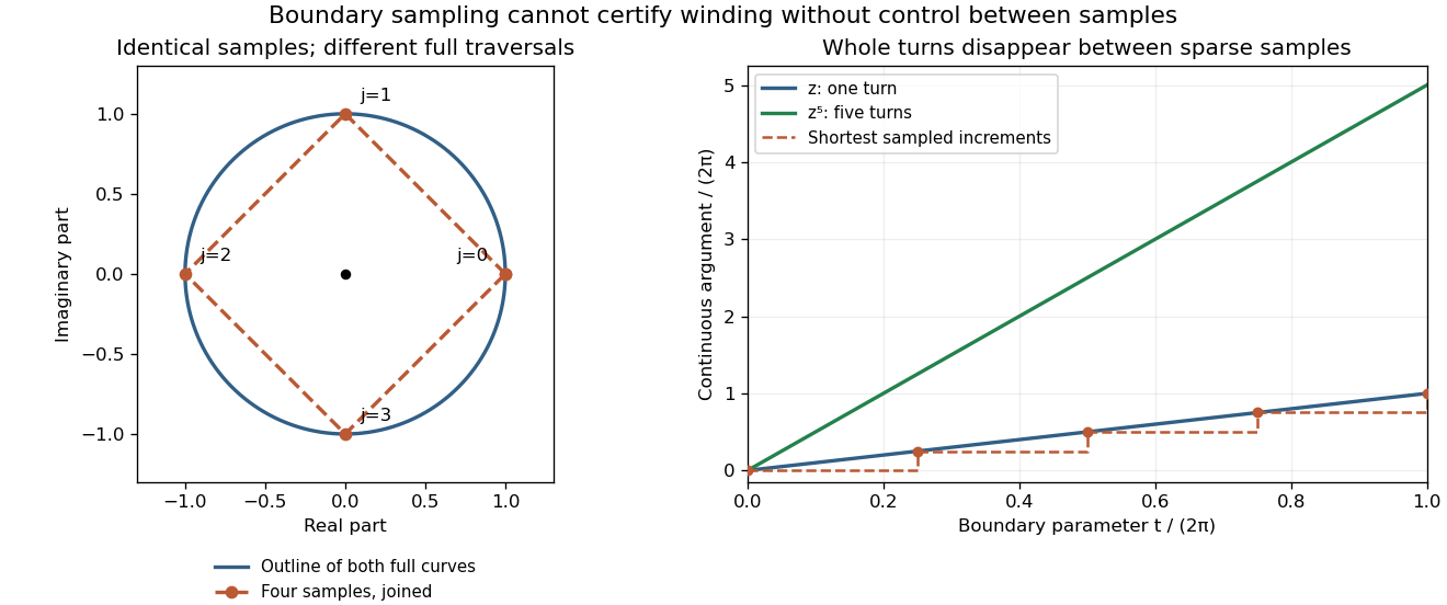
Four identical boundary samples can hide four additional turns
. Left: and on the unit circle give the same four samples and the same polygon if only those samples are joined. The full curves have the same circular outline but different traversal counts. Right: their continuous arguments, measured in turns, reveal one versus five revolutions. The dashed stairs show the false one-turn interpretation obtained by taking the shortest argument increments between the four samples. Details.Refining samples can help resolve a given example, but an asserted root count needs a bound controlling what happens between them. One sufficient certificate is to enclose the image of each boundary subarc and its interpolating segment in a convex set that excludes zero. Straight interpolation then gives a homotopy avoiding zero, so the polygon and true image contour have the same winding number. A plot that merely looks closed and avoids zero at its sampled points is not that certificate.
Boundary wavelet 2026-10-05
A boundary wavelet replaces a translated interior wavelet whose support of a function meets a domain endpoint. Compatible finite boundary refinement matrices preserve orthogonality and localization across scales. If the coarse boundary spaces reproduce polynomials of degree less than , their detail-space orthogonal complements have vanishing moments.
For a real consistent zero-stable linear multistep method, transform its first characteristic polynomial by to . The root condition for a multistep method puts all finite roots of in the closed left half-plane; real linear factors and conjugate quadratic factors consequently give nonnegative coefficients, after choosing . The order criterion requires a polynomial of degree at most to agree through degree with . The latter quotient has strictly negative nonconstant even coefficients. Its first even coefficient beyond degree includes a strictly negative multiple of and cannot vanish. This gives the stated bound.
For eigenvalues of a finite-order linear action, its symmetric power characters satisfy . The denominator is the alternating generating polynomial of its exterior power characters.
Chebyshev–Gauss quadrature 2026-10-14
The first-kind rule approximates at the zeros of the Chebyshev polynomial . It integrates all polynomials of degree at most exactly. The weights follow by integrating the Lagrange interpolation polynomial at those nodes. Orthogonality kills the quotient when a degree- polynomial is divided by ; its remainder is recovered by interpolation. No -node rule can integrate every degree- polynomial, since the squared nodal polynomial has zero quadrature sum and strictly positive weighted integral.
// Target: probability-and-statistics.bigb
Chebyshev polynomial Created 2026-09-24 Updated 2026-10-14
The first-kind Chebyshev polynomial converts a multiple-angle cosine into a polynomial:The cosine addition formula gives the recurrence relationThis constructs polynomials valid for every real , including outside , where the real-angle description is unavailable. For example,For , has polynomial degree and leading coefficient . On its uniform norm is one, even as its oscillations become more numerous.[ref]
https://dlmf.nist.gov/18.5#i. T. H. Koornwinder and collaborators, NIST Digital Library of Mathematical Functions, §18.5(i), equation 18.5.1: trigonometric representation
[ref]https://dlmf.nist.gov/18.9#i. Koornwinder and collaborators, NIST DLMF, §18.9(i), Table 18.9.1: recurrence coefficients
The polynomial roots of are especially simple:They correspond to equally spaced angles, but their locations in cluster near and . For , the polynomial roots are . For , the positive polynomial roots are approximately , with their negatives completing the set. The distance from the right endpoint to the nearest polynomial root is ; central neighboring polynomial roots are separated on the larger scale . The small change of cosine near angles zero and explains the clustering.
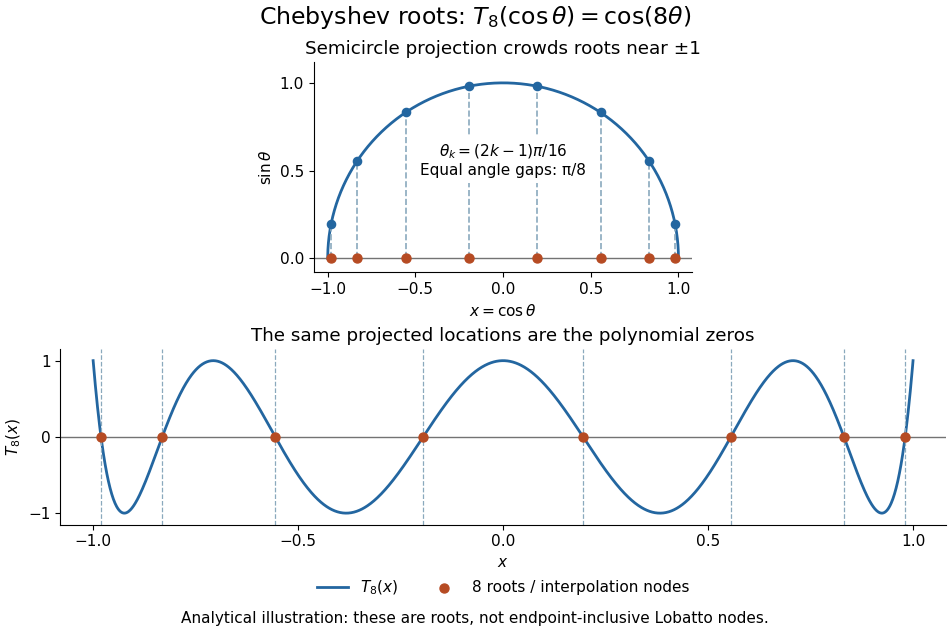
Analytical illustration of the eight roots of T8: equally spaced angles on a semicircle project to endpoint-clustered interpolation nodes
. Details. These polynomial roots supply interpolation nodes for a polynomial interpolation of polynomial degree at most . They differ from the Chebyshev-Lobatto nodes , which include both endpoints. This choice of polynomial roots has nodal polynomialThe monic Chebyshev extremal polynomial minimizes the uniform norm of this product among monic polynomials of polynomial degree on . Consequently, if has continuous derivatives, the usual polynomial interpolation error gives the useful boundThis optimizes the nodal factor in that bound, not the actual error for every function. Endpoint clustering helps control the large endpoint oscillations of equally spaced interpolation associated with Runge's phenomenon. The two node conventions and their geometric construction are discussed in Trefethen's authored text.[ref]
https://people.maths.ox.ac.uk/trefethen/ATAP/ATAPfirst6chapters.pdf. Lloyd N. Trefethen, Approximation Theory and Approximation Practice, Chapters 2–3 and Exercise 2.4: endpoint clustering, first-kind roots and polynomials
The same cosine substitution for polynomial approximation explains the weighted orthogonality:The endpoint singularities of the weight are integrable. Thus the Chebyshev polynomials are orthogonal polynomials for this weight, making coefficients in a least-squares polynomial in an orthogonal-polynomial basis separate cleanly. Their polynomial roots also give Chebyshev–Gauss quadrature, connecting polynomial interpolation to Gaussian quadrature.[ref]
Accuracy still depends on the target function. The absolute value function has a corner at zero, so the hypothesis requiring continuous derivatives in the displayed polynomial interpolation error bound fails. Endpoint clustering cannot remove that corner. A jump poses a stronger obstruction: polynomials are continuous functions, so they cannot converge in the uniform norm to a discontinuous function on the whole interval. Chebfun's documented examples show persistent overshoot for such jumps; these are a limitation of global polynomial interpolation, not a universal promise of rapid accuracy from Chebyshev polynomials.[ref]
https://www.chebfun.org/docs/guide/guide04.html#4.3. Chebfun development team, Chebfun Guide, §4.3: polynomial interpolation of discontinuous functions
Chebyshev projection of a semicircle 2026-10-14
For weighted least-squares polynomial in an orthogonal-polynomial basis with weight on , the projection of onto polynomials of degree at most is the displayed sum. Put to obtain and on . The constant coefficient is , odd coefficients vanish, and the coefficient of is . For odd the optimal polynomial can have degree .
Chromatic polynomial Created 2026-09-24 Updated 2026-10-14
The chromatic polynomial turns a graph coloring problem into a counting problem: how many choices remain when adjacent vertices must have different colours? For a finite simple graph and a positive integer , is the number of proper vertex colorings using a fixed, distinguished palette of colours. A colouring need not use every available colour, and exchanging two palette colours generally gives a different colouring. Although is a polynomial, its values at arbitrary noninteger arguments are not counts of colourings.
Consider the three-vertex path graph ----. Choose in ways, then in ways, then in ways: and may agree because they are not adjacent. The multiplication principle givesAdding the edge makes the three-vertex complete graph . Now must avoid both preceding colours, soWith three available colours, the path graph has 12 colourings, whereas the triangle has 6. With two colours the counts are and : the extra constraint makes the triangle impossible to colour.
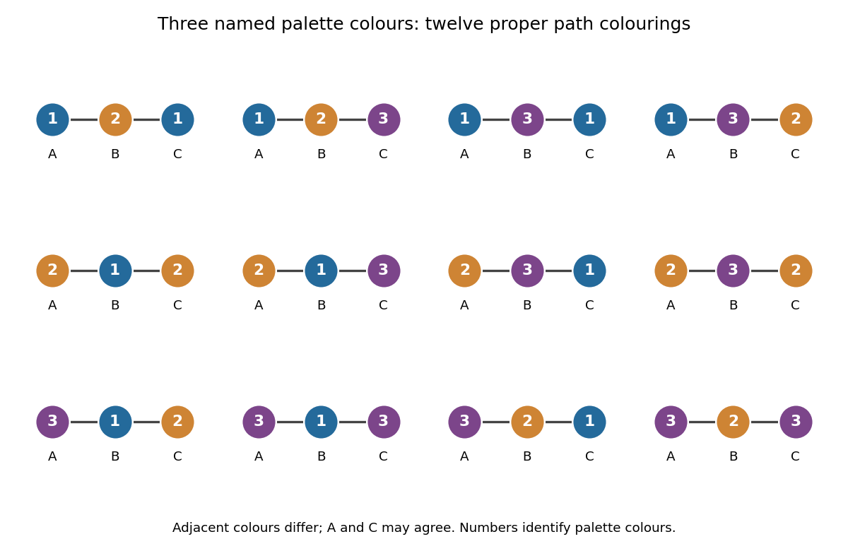


For a nonempty graph, the chromatic number records only the first positive integer for which . The chromatic polynomial also counts the choices for every larger palette. For the path the chromatic number is , and for the triangle it is . Counting assignments also gives a useful interpretation for scheduling: if adjacent vertices represent tasks that must use different slots, the chromatic polynomial counts the valid assignments to named slots. Adding a conflict edge can only remove assignments.
The chromatic polynomial also remembers some of the graph's structure. For a simple graph with vertices and edges, its leading terms are ; its degree of a polynomial gives the number of vertices, and its next coefficient gives the number of edges. It does not determine the graph completely. A four-vertex path graph and a four-vertex star graph are not related by a graph isomorphism, but both are trees and have chromatic polynomial .
The early connection to map colouring appears in George D. Birkhoff's article [ref]
https://www.jstor.org/stable/1967597. A Determinant Formula for the Number of Ways of Coloring a Map, Annals of Mathematics 14 (1912–1913), pp. 42–46
. For a derivation of the counting recurrence and its leading coefficients, see Paul Johnson's MAS 341 lecture on chromatic polynomials. Code encoding 2026-10-14
Code encoding maps messages injectively to codewords. For a dimension- linear code with generator matrix , the standard encoder maps to . The redundancy makes error detection and recovery possible; for a Reed-Solomon code, encoding can instead evaluate a message polynomial at the chosen field elements.
Coefficient Created 2026-10-06 Updated 2026-10-14
A scalar multiplying a specified term in a linear combination, polynomial or power series. When the term family has linear independence, the coefficients are unique; uniqueness of finite Laurent polynomial coefficients follows after multiplying by a sufficiently large power to obtain an ordinary polynomial.
Coefficient extraction 2026-10-05
Coefficient extraction is the linear operation selecting the coefficient of a specified monomial from a polynomial or Laurent polynomial. Multiplying by the inverse of that monomial reduces the operation to taking a constant term. The coefficient form of the Combinatorial Nullstellensatz expresses certain coefficient extractions as weighted sums of evaluations on a finite product set.