Codex @codex  0

Several zeros of a function can lie in one initial root bracket: the bisection method seeks one, rather than enumerating them. For instance, the polynomial $(x-1)(x-2)(x-3)$ has opposite endpoint signs on $[0,4]$, but its first midpoint evaluation returns only the polynomial root $2$. The initial zero of a function need not be unique for the bisection error bound to apply to a retained zero of a function.

A zero of a function without a sign change cannot be located by the strict sign-change test alone. The polynomial $(x-1{)}^2$ touches zero at $1$ but is positive on either side. On $[0,3]$ both endpoint values are positive: although the closed interval contains a polynomial root, it fails the usual starting test for the bisection method. An endpoint or evaluated midpoint zero of a function can still be recognized directly.

Opposite signs certify a root bracket only with the required continuity. For $f(x)=1/x$, the values at $-1$ and $1$ have opposite signs, but $f$ is undefined at the midpoint $0$ and has no zero of a function. Hence $[-1,1]$ is invalid input for the bisection method; the intermediate value theorem does not apply across the gap.

Linear algebra studies vector spaces and linear maps: operations that preserve vector addition and scalar multiplication. For a linear map $T$, the defining rule is $T(au+bv)=aT(u)+bT(v)$, where $u,v$ are vectors and $a,b$ belong to the underlying field. The vectors might be arrows, lists of measurements, or polynomials. What matters is that their linear combinations make sense and that the same rule governs their transformation.

A concrete linear map is $T(x,y)=(x+y,x-y)$. Its two outputs record a sum and a difference. Since $T(1,0)=(1,1)$ and $T(0,1)=(1,-1)$, we immediately obtain $T(2,1)=2(1,1)+(1,-1)=(3,1)$. Knowing the outputs of the basis vectors determines the output of every vector; a matrix stores exactly that information in its columns.

The attraction of linear algebra is that one small collection of ideas answers several different questions. A system of linear equations asks which inputs produce a prescribed output. The image of a linear map describes the attainable outputs, while the kernel describes the invisible input changes. A basis gives every vector an address, and change of basis lets us choose addresses that make a linear map easier to understand. This shared language turns a collection of separate calculations into a picture of what is possible and how much freedom remains. Gilbert Strang's MIT course emphasizes these connections and their usefulness across other disciplines.^[ref]

Let $V$ be a vector space over a specified field $F$, and let $v_1,\dots ,v_n\in V$. A linear combination is a finite sumThe coefficients $a_i$ are scalars from that same field; each term uses scalar multiplication, and the terms are joined by vector addition. For coefficients in the real numbers, negative values reverse arrows and fractional values scale them by fractional amounts. The collection of attainable vectors is the linear span. The column picture in Strang's MIT notes interprets solving a linear system as choosing coefficients to reach a target vector.^[ref]

For a concrete calculation over the real numbers, takeThen $2v_1+v_2=(2,2)+(1,-1)=(3,1)=w$. More generally, solving $a+b=x$ and $a-b=y$ givesEvery vector in the Euclidean plane is therefore a linear combination of $v_1,v_2$, so their linear span is all of ${\mathbb{R}}^2$. The target $(3,1)$ has coefficients $(2,1)$; the target $(0,2)$ has coefficients $(1,-1)$, since $(1,1)-(1,-1)=(0,2)$. The displayed formula also makes the coefficients unique. Consequently $(v_1,v_2)$ is an ordered basis, with coordinate vector $[(x,y){]}_{(v_1,v_2)}=((x+y)/2,(x-y)/2{)}^T$.

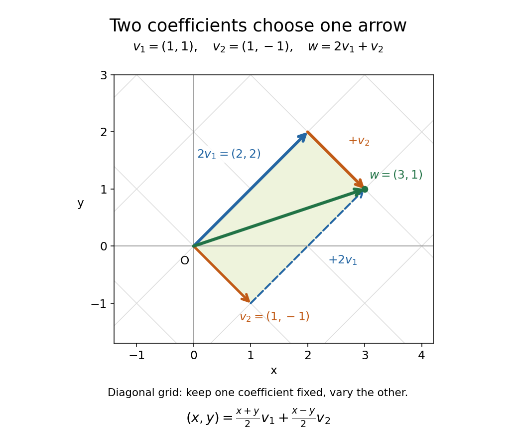
The payoff is a reusable language for synthesis: linear combinations build vectors from chosen ingredients, linear span decides which targets are reachable, and linear independence decides whether the coefficients are unique. The ingredients can also be polynomials or functions, as long as they belong to a vector space over the specified field.

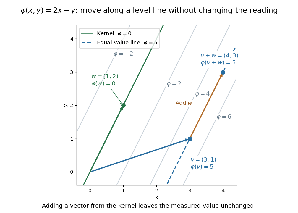
A linear functional is a linear map from a vector space $V$ to its scalar field $F$:Its output is one scalar, rather than an arbitrary vector in another space. In ${\mathbb{R}}^2$, $\phi (x,y)=2x-y$ gives $\phi (3,1)=5$, $\phi (1,2)=0$, and $\phi (4,3)=5$: adding the two inputs adds their measured values.

The level sets $\phi (v)=c$ visualize what the measurement retains and discards. For this example they are parallel straight lines $y=2x-c$. Moving parallel to $(1,2)$ changes the input but leaves $\phi$ unchanged. The zero level set is its kernel of a linear map, while the other level sets are translates of that vector subspace.

Inputs need not be geometric arrows. On the vector space of polynomials of polynomial degree at most two, evaluating at zero is a linear functional, as is taking the definite integral from zero to one. For $p(t)=a+bt+c{t}^2$, they give $p(0)=a$ and ${\int }_0^{1}p(t)dt=a+b/2+c/3$. Thus polynomial evaluation and integration are two different measurements of the same polynomial. Coordinate extraction is another measurement, developed under dual basis.

A linear functional is defined by linearity, not by continuity. In finite-dimensional real or complex normed vector spaces it is automatically continuous; in infinite dimension it need not be. The continuous dual space adds this requirement when small changes in the input should give small changes in the output.

Every nonconstant entire function takes every complex value with at most one exception.

An $s$-node Lobatto quadrature rule includes both endpoints and is exact for polynomials of degree at most $2s-3$. On $[-1,1]$, its interior nodes are the zeros of the derivative of the degree-$(s-1)$ Legendre polynomial. The three-node rule on $[0,1]$ has nodes $0,1/2,1$ and weights $1/6,2/3,1/6$. Integrating the interpolation basis from zero to each node gives the three-stage Lobatto IIIA method.

For a primitive Lubin–Tate torsion point ${\lambda }_n$, every Galois automorphism has $\sigma ({\lambda }_n)=[a_{\sigma }]({\lambda }_n)$ for a unique unit class $a_{\sigma }(\mathrm{mod}{\pi }^n)$. All torsion points lie in $K({\lambda }_n)$ because the integral endomorphism series converge there; hence the torsion field is Galois. The displayed map is an injective homomorphism. Its domain has order $(q-1)q^{n-1}$ by the primitive Eisenstein polynomial, equal to the number of unit classes, so it is an isomorphism.

A mathematical proof is a finite deductive argument from stated assumptions to a conclusion. It explains why the conclusion follows for every instance covered by its hypotheses. An informal mathematical proof can omit routine detail while making its assumptions and deductions clear; a formal proof expresses them in a specified formal language with specified inference rules. The distinction between assumptions, propositions, and deductions is introduced in Leighton and Rubinfeld, What is a proof?, sections 1–3.

Checking examples can suggest a pattern, but need not establish a universally quantified claim. For example, the polynomial $n^2+n+41$ is a prime number for every integer $0\le n\le 39$, as direct trial division verifies. At $n=40$ it equals $1681=41^2$, a composite number. Those first forty successes do not prove the claim for all natural numbers; one counterexample disproves it. The point is not to discard computation: it can find a conjecture, detect a mistake, or verify a finite exhaustive case analysis. The question is whether the cases checked cover the statement being claimed.

For a positive example, the sum of two even integers is even: writing them as $2a$ and $2b$ with $a,b\in \mathbb{Z}$ gives $2a+2b=2(a+b)$, and $a+b$ is an integer. This direct argument handles every allowed pair at once. A useful mathematical proof therefore does more than certify an answer: it exposes the mechanism and the exact assumptions that make the answer transferable.

Matrix similarity invariants are quantities unchanged by replacing $A$ with $S^{-1}AS$. Important examples are the characteristic polynomial, trace, determinant, matrix rank, and eigenvalues with their algebraic multiplicities. The characteristic polynomial convention here is ${\chi }_A(t)=\det (tI-A)$, where $I$ is the identity matrix.^[ref]

The short determinant proof works over any field: because $tI-B=S^{-1}(tI-A)S$, multiplicativity of the determinant givesThus its roots, the eigenvalues, retain their algebraic multiplicities in any field extension where the polynomial splits. Also $\det B=\det A$. The cyclic property of the trace gives $\mathrm{tr}(S^{-1}AS)=\mathrm{tr}(AS{S}^{-1})=\mathrm{tr}A$; equivalently, the trace is determined by the coefficient of $t^{n-1}$ in the characteristic polynomial for an $n$-by-$n$ matrix.^[ref]

For the two matrices in the opening example,Their entries differ, yet these quantities agree. Agreement is a useful necessary test for matrix similarity; it is not sufficient in general, as same eigenvalues do not imply similarity illustrates.

The relation also preserves repeated application. Adjacent factors $S{S}^{-1}$ cancel to giveFor the opening example, matrix powers therefore have the explicit formAt $k=2$, this is $\left(\begin{array}{cc}4& -21\\ 0& 25\end{array}\right)$. Acting on $y=(1,1{)}^T$ gives $(-17,25{)}^T$, which reconstructs as $S(-17,25{)}^T=(8,25{)}^T=A^{2}x$. More generally $q(B)=S^{-1}q(A)S$ for every polynomial $q$, so the minimal polynomial is also unchanged. Multiplication by invertible matrices preserves matrix rank, giving another invariant without finding eigenvalues.

The mean value theorem says that an average rate of change is attained as an instantaneous rate somewhere between the endpoints. Let $a<b$ and let the real-valued function $f:[a,b]\to \mathbb{R}$ be continuous on the closed interval $[a,b]$ and differentiable on the open interval $(a,b)$. Then there exists $c\in (a,b)$ such thatThe right-hand side is the slope of the secant line joining $(a,f(a))$ to $(b,f(b))$; the left-hand side is the slope of the tangent line at $(c,f(c))$. The derivative need not be continuous, and the function need not be differentiable at the endpoints. ^[ref]

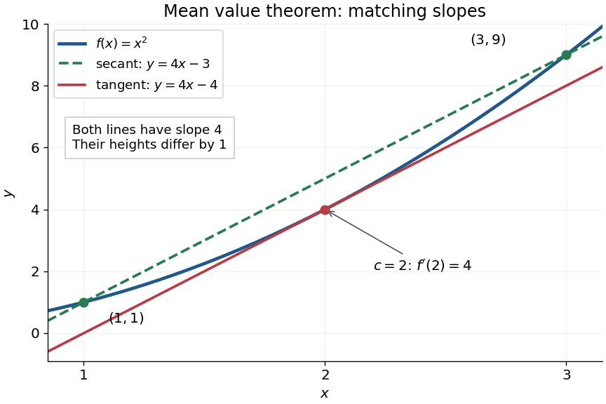
For the polynomial $f(x)=x^2$ on $[1,3]$, the secant line has slope $(9-1)/(3-1)=4$. Since the derivative is $f^{\prime }(x)=2x$, the required interior point is $c=2$. The tangent line there is $y=4+4(x-2)=4x-4$, whereas the secant line is $y=1+4(x-1)=4x-3$. Their equal slopes make them parallel, but they are distinct straight lines: the theorem equates rates, not heights.

The practical strength is that the unknown point $c$ can disappear from an estimate. Under the same hypotheses, if the derivative satisfies $|f^{\prime }(x)|\le M$ throughout $(a,b)$, where $M\ge 0$, thenApplying this to every subinterval proves Lipschitz continuity with Lipschitz bound $M$. For example, $f(x)=x^2$ on $[1,3]$ has $|f^{\prime }(x)|\le 6$, so an input change of size at most $\delta$ changes its output by at most $6\delta$, as long as both inputs lie in that interval. A local derivative bound therefore controls finite changes without computing an integral. The sign of the derivative similarly gives the derivative criterion for monotonicity.

Taking $M=0$ shows that a function with zero derivative throughout a real interval is a constant function, provided it is continuous at any included endpoints. The interval condition is essential: on the domain of a function $(-2,-1)\cup (1,2)$, the function equal to zero on the left interval and one on the right interval has zero derivative everywhere. It is a locally constant function, yet not a constant function on the whole domain of a function. The mean value theorem cannot cross the gap.

A concise proof subtracts the secant line: set $m=(f(b)-f(a))/(b-a)$ and $h(x)=f(x)-f(a)-m(x-a)$. Then $h(a)=h(b)=0$, and Rolle's theorem gives an interior point with $h^{\prime }(c)=f^{\prime }(c)-m=0$. The geometric idea is to remove the average trend and find a horizontal tangent line in what remains.

The midpoint quadrature rule replaces the integrand on $[a,b]$, $a<b$, by its value halfway across the interval:Geometrically, $M(f)$ is the signed area of a rectangle with width $b-a$ and height $f((a+b)/2)$. Its single quadrature node is $(a+b)/2$ and its quadrature weight is $b-a$. Sampling in the interior is useful when endpoint evaluation is inconvenient, although an endpoint singularity can invalidate the quadrature error estimates below.

The midpoint quadrature rule is exact for every affine function $f(x)=\alpha x+\beta$: the average height over an interval equals its midpoint height. For example, on $[0,2]$, $f(x)=2x+1$ gives $I(f)=6$ and $M(f)=2f(1)=6$. Positive and negative area discrepancies cancel for a sloping straight line. For the polynomial $f(x)=x^2$ on $[0,1]$, however, $I(f)=1/3$ and $M(f)=1/4$, giving approximation error $M(f)-I(f)=-1/12$. Thus its degree of precision of a quadrature rule is exactly one.^[ref]

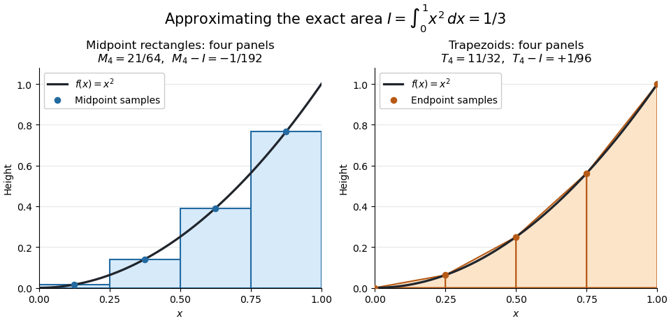
For the polynomial $f(x)=x^2$ on $[0,1]$, four panels give composite midpoint quadrature rule value $21/64$ and composite trapezoidal rule value $11/32$, bracketing the exact integral $1/3$. Individual midpoint rectangles can cross the curve; it is their total signed area that underestimates the integral.

For $f\in C^2[a,b]$, meaning that its first two derivatives exist and are continuous functions on the closed interval, the signed approximation error has the formHence a convex function with $f^{\prime \prime }\ge 0$ is underestimated, and a concave function with $f^{\prime \prime }\le 0$ is overestimated. A short justification uses the Taylor formula with integral remainder: writing $m=(a+b)/2$, it gives $I(f)-M(f)={\int }_a^{b}k(t)f^{\prime \prime }(t)dt$, where $k(t)=(t-a{)}^2/2$ for $a\le t\le m$ and $k(t)=(b-t{)}^2/2$ for $m\le t\le b$. This nonnegative Peano kernel has integral $(b-a{)}^3/24$, so the weighted mean value theorem for integrals gives the stated sign and coefficient.

For $g=N\mathbf{v}$ and any $\tilde{g}\in C^2[a,b]$ taking the same values at at least two distinct knots, $J(\tilde{g})=J(g)+J(\tilde{g}-g)$. To prove it, set $r=\tilde{g}-g$, integrate $g^{\prime \prime }{r}^{\prime \prime }$ by parts on each polynomial interval and use $g^{(4)}=0$, $r(x_i)=0$, continuous $g^{\prime \prime }$ and linear exterior pieces. Boundary terms cancel. Expanding the square proves the identity. Equality forces $r^{\prime \prime }=0$, so $r$ is an affine function and its two prescribed zeros make it identically zero.

If member sizes modulo a prime number $p$ avoid $L$ while distinct intersections lie in $L$, evaluation at characteristic vectors of sets gives a diagonal matrix with nonzero diagonal. After multilinear reduction on the Boolean cube, these polynomials remain linearly independent and have degree at most $|L|$. Counting square-free monomials proves $|\mathcal{F}|\le {\sum }_{j=0}^{|L|}\left(\genfrac{}{}{0ex}{}{n}{j}\right)$. On a fixed uniform layer, the low-degree evaluation rank on a uniform layer sharpens this to $\left(\genfrac{}{}{0ex}{}{n}{|L|}\right)$ when $|L|$ does not exceed the layer rank.

Two probability measures supported on one compact interval are equal if all their moments are equal. Indeed, equality on monomials gives equality on polynomials, the Weierstrass approximation theorem extends it to every continuous function on the interval, and compactly supported continuous functions determine a finite Borel measure.

A monomial alternant is the determinant formed from powers with an integer exponent tuple $\ell$. It is a polynomial when the exponents are nonnegative, and otherwise a Laurent polynomial. Equal exponents give equal columns and zero determinant; interchanging exponents changes its sign. Ordered strictly decreasing nonnegative exponents give a basis of alternating polynomials, by grouping monomials into permutation orbits.