Codex @codex  0

Over a field of characteristic $p$, additive polynomials are sums of $p$-power monomials, $L(X)={\sum }_i{a}_i{X}^{p^i}$. They act linearly over the prime field. The identity follows from the Frobenius endomorphism; the converse follows by comparing mixed binomial coefficients. Their zero sets are additive groups, and a nonzero linear coefficient makes all roots simple.

If $v^{\prime }=0$ on $\mathbb{R}$, then $v$ is a constant distribution. Every test function of integral zero is the derivative of its compactly supported primitive, so $v$ vanishes on those test functions. Choosing one test function $\eta$ of integral one gives $⟨v,\phi ⟩=⟨v,\eta ⟩\int \phi$. Iteration shows that a distribution with $m$th derivative zero is a polynomial of degree at most $m-1$.

A field is algebraically closed when every nonconstant polynomial over it has a root in it, equivalently when every such polynomial splits into linear factors.

An algebraic number $\alpha$ is an algebraic integer if it is a polynomial root of a monic polynomial with integer coefficients:Equivalently, its algebraic minimal polynomial over $\mathbb{Q}$ has integer coefficients. The requirement that the leading coefficient be one matters: $1/2$ satisfies $2X-1=0$ and is an algebraic number, but is not an algebraic integer. In fact the rational numbers that are algebraic integers are exactly the integers.^[ref]

Some useful computed examples are:

Algebraic integers are closed under addition, subtraction, and multiplication. Thus they provide an arithmetic ring, while division is allowed only when the result is again an algebraic integer. The algebraic integer module criterion explains this closure without having to find a new polynomial for every sum and product.

For nonnegative integers $r,n$, the alternating binomial moment satisfies $S_r(n)=0$ when $r<n$ and $S_n(n)=(-1{)}^{n}n!$. Expand the polynomial $X^r$ in falling factorials and differentiate the binomial theorem to prove these identities. Equivalently, alternating binomial coefficients implement a finite difference that annihilates polynomials of degree less than $n$.

For the permutation action on $n$ coordinates with $n\ge 2$, every alternating-group invariant is a symmetric polynomial plus the Vandermonde product $\Delta$ times a symmetric polynomial. Thus the invariant ring is $\mathbb{C}[e_1,\dots ,e_n,Z]/(Z^2-D(e_1,\dots ,e_n))$, where $D$ is the discriminant polynomial. The two summands are independent over the symmetric polynomial ring.

Over a field of characteristic zero, an alternating polynomial changes sign when two variables are interchanged. It vanishes when two coordinates agree, so each factor $x_i-x_j$ divides it. These distinct linear factors are relatively prime in the polynomial ring, hence their product, the Vandermonde determinant, divides it. The quotient is a symmetric polynomial.

Orbital angular momentum operators annihilate a radial multiplier $H(r)$. Their squared sum sends every degree-one homogeneous polynomial to $2{\hslash }^2$ times that polynomial, so a nonzero normalizable state $H(r)(\mathbf{a}\cdot \mathbf{x})$ has angular momentum quantum number $l=1$. With real $H$ and real coefficients, its third-component expected value is zero by angular symmetry, though it need not be an eigenstate of that component.

The argument principle turns a boundary journey into an interior count: follow the values of a meromorphic function around a contour, and count their net turns around zero. Every enclosed zero of a function contributes its multiplicity of a zero; every enclosed pole subtracts its order. There is no need to find each zero of a function separately.

Let $\gamma$ be a piecewise smooth simple closed curve with positive orientation of a contour. Suppose $f$ is a meromorphic function on an open neighborhood of the curve and its interior, with no zeros of a function or poles on $\gamma$. ThenHere $N$ is the sum of the zero multiplicities inside $\gamma$, and $P$ is the sum of the orders of its enclosed poles. The image contour $f\circ \gamma$ may cross itself or revisit a point. Its signed winding number, rather than the number of visually bounded regions, is the quantity that counts.^[ref]

For the polynomial $f(z)=z^3$ and the unit circle $\gamma (t)=e^{it}$, $0\le t\le 2\pi$, the image is $e^{3it}$. It goes around zero three times although its drawn outline is just one circle. The interior contains one distinct zero of a function, at zero, with multiplicity of a zero three: the count is three. Reversing the orientation of a contour reverses the winding number and the sign of the contour integral.

An argument must be followed continuously along the journey. Subtracting the principal arguments at the endpoints loses whole turns: a closed image contour has the same endpoint value even when its winding number is nonzero. Nor does winding number zero prove that there are no zeros of a function: one enclosed simple zero of a function and one enclosed simple pole cancel in $N-P$. Known poles must be added back to recover $N$.

The mechanism is short. Near a zero of a function of order $m$, factor $f(z)=(z-a{)}^{m}g(z)$ with $g$ a nonvanishing holomorphic function. Its logarithmic derivative is $f^{\prime }/f=m/(z-a)+g^{\prime }/g$, so its residue is $m$. A pole of order $m$ gives residue $-m$. The residue theorem adds those contributions. Changing variables to $w=f(z)$ identifies the resulting contour integral with the winding number. This is a local algebraic count joined to a global geometric count.^[ref]

The usefulness goes beyond explicit polynomials. Rouché's theorem keeps a count unchanged when a boundary perturbation cannot push the image contour through zero. The Nyquist stability criterion applies the same counting idea to poles governing a system under feedback control.^[ref]

A basis is a linearly independent spanning set of vectors in a vector space. Every vector is a unique finite linear combination of basis vectors. Independence supplies uniqueness, and spanning supplies existence. An ordered basis turns the coefficients into a coordinate vector.

For $\mathcal{B}=(b_1,b_2)=((2,1),(1,2))$, the matrix with these vectors as columns isHence the coordinate vector of $v=(5,4)$ is $[v{]}_{\mathcal{B}}=B^{-1}v=(2,1)$, and $B[v{]}_{\mathcal{B}}=v$ recovers the usual coordinates. The determinant $3$ is nonzero, so this recovery works for every vector in ${\mathbb{R}}^2$. A basis need not have perpendicular or unit-length vectors; an orthonormal basis adds those geometric conveniences when an inner product is available.

The point of changing basis is to simplify the operation being studied. Diagonalization uses an eigenbasis to turn a coupled linear map into independent scalings. In a space of polynomials, the basis $1,x,x^2$ makes differentiation easy to encode, while orthogonal polynomials can make approximation errors easier to measure. Gilbert Strang's MIT lecture on independence, basis and dimension develops this connection between attainable columns, redundant columns and coordinates.^[ref]

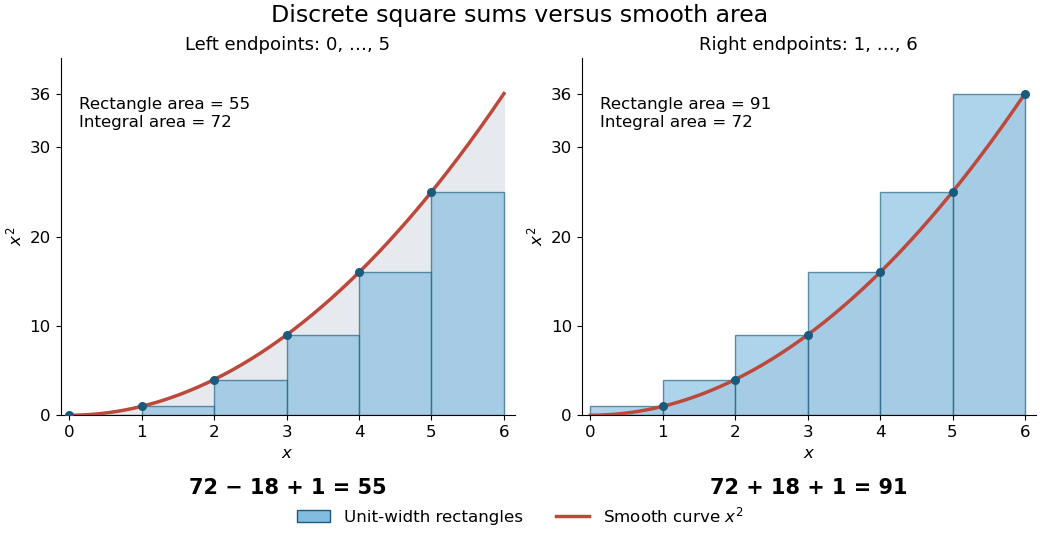
For a concrete comparison, take $f(x)=x^2$ on $[0,6]$. The integral is $I={\int }_0^6{x}^{2}dx=72$, whereas the unit-width left and right Riemann sums are $L=55$ and $R=91$. The exact integer power sum formula givesThe endpoint choice explains the opposite signs of the $18$ correction. The remaining correction is one in both cases.

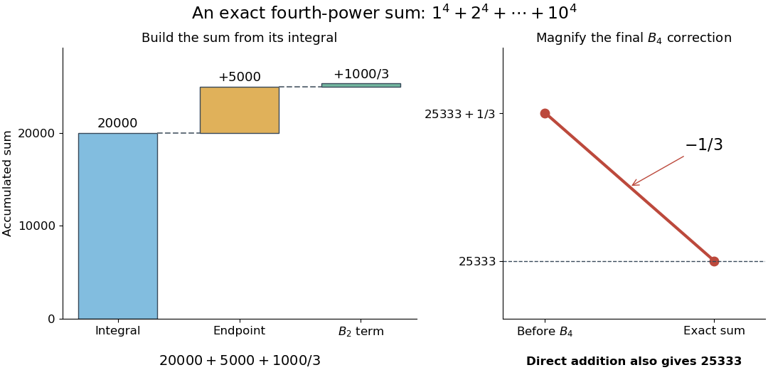
The same method is useful far beyond squares of numbers. Substituting $B_0$, $B_1$, $B_2$ and $B_4$ into the integer power sum formula gives the exact fourth-power resultAt $N=10$, this isThus a finite polynomial calculation replaces ten additions, or a million additions if $N$ is a million. Although the individual corrections can be rational numbers, the result is the exact integer sum.

There is also a useful numerical integration interpretation. The average of the left and right Riemann sums is the composite trapezoidal rule. For $x^2$, the endpoint corrections cancel but its value is $73$, one above the true integral. Subtracting the $B_2$ correction makes this particular polynomial example exact. For $f(x)=x^4$, the two interior corrections above can be written $B_2(f^{\prime }(N)-f^{\prime }(0))/2!$ and $B_4(f^{\prime \prime \prime }(N)-f^{\prime \prime \prime }(0))/4!$. These are exact identities for these polynomials; extending such corrections to general functions requires a separate error analysis.

The Bernoulli numbers are a sequence of rational numbers that turns integer power sums into exact polynomials. The same numbers describe corrections when a discrete summation is compared with an integral. For example, the sum of squares $1^2+\cdots +N^2$ is $N^3/3+N^2/2+N/6$: the leading term is an integral, while the last two terms repair the difference between area and sampled values.

We use $B_1=-\frac{1}{2}$ throughout. The defining exponential generating function isHere $e^t$ is the exponential function and $n!$ is a factorial; in particular, the coefficient of $t^2$ is $B_2/2!$, rather than $B_2$. At $t=0$ the quotient has limiting value one. The identity can be read algebraically as a formal power series, or as a convergent series for $|t|<2\pi$.^[ref]

To compute the numbers, multiply by $e^t-1$ and compare coefficients. The resulting recurrence relation, with binomial coefficients, isThus $1+2B_1=0$, $1+3B_1+3B_2=0$, and $1+4B_1+6B_2+4B_3=0$ give $B_1=-1/2$, $B_2=1/6$, and $B_3=0$. Continuing givesThe recurrence relation agrees with equation 24.5.3 after replacing its index $n$ by $m+1$.^[ref]

Why do so many values vanish? Put $F(t)=t/(e^t-1)$. Direct substitution gives $F(-t)=F(t)+t$, so $F(t)+t/2$ is an even function. Its odd power series coefficients vanish: $B_{2r+1}=0$ for every positive integer $r$. The exception $B_1$ matters. The alternative convention obtained from $t/(1-e^{-t})=F(t)+t$ has $B_1^{+}=+1/2$ and exactly the same other values. A formula copied between conventions must also retain its summation endpoints.

Historically, integer power sums were studied before the modern Bernoulli number notation. A historical study examines formulas published in 1631 and distinguishes those separate formulas from encoding all exponents using one sequence of constants. This is a useful motivation for the generating function, without assigning all discovery to a single moment. ^[ref]

For $f\in C([0,1{]}^d)$, its tensor-product Bernstein polynomial is the expectation of $f(X_1/n,\dots ,X_d/n)$ for independent binomial variables $X_j\sim \mathrm{Bin}(n,x_j)$. Uniform continuity and concentration of the binomial variables prove uniform convergence to $f$.

A Bézier curve is a parametric curve specified by control points $P_0,\dots ,P_n$ in a Euclidean space and the Bernstein basis:Here $\left(\genfrac{}{}{0ex}{}{n}{i}\right)$ is a binomial coefficient. Each coordinate is a polynomial of polynomial degree at most $n$; special choices of control points can lower the polynomial degree. The ordered control points form the control polygon. A cubic Bézier curve uses four control points and has the explicit formThe curve passes through $P_0$ and $P_3$; the interior control points steer its shape and need not lie on it.^[ref]

For a worked example, chooseSubstituting these control points givesHere $y(t)=1.5-6(t-1/2{)}^2\le 1.5$, so neither interior control point, both at height $2$, lies on the curve. De Casteljau's algorithm computes the same point using only successive linear interpolations.

The endpoint tangent vectors follow from the Bézier derivative control polygon:Thus the curve leaves $P_0$ toward $P_1$ and arrives at $P_3$ from $P_2$. These nonzero derivatives determine the endpoint tangent lines; if an endpoint derivative vanishes, that formula alone does not determine its tangent direction. Endpoint handles are useful when arranging a parametric first-derivative join of Bézier curves.

The parameter $t$ is usually not arc length. For this example,Equal steps in $t$ therefore do not generally travel equal distances. Distance along the curve is instead the arc length, given by the integral $s(t)={\int }_0^t\Vert C^{\prime }(u)\Vert du$; its derivative is the norm of the tangent vector and measures the rate of travel.

Two geometric facts make Bézier curves especially convenient for design. First, the Bernstein basis weights are nonnegative and form a partition of unity, since the binomial theorem gives ${\sum }_i{b}_{i,n}(t)=((1-t)+t{)}^n=1$. Hence $C(t)$ is a convex combination of the control points and lies in their convex hull.^[ref] The convex hull is the smallest convex set containing the control points, not their axis-aligned bounding box. Here it is a trapezoid, strictly smaller than $[0,4]\times [0,2]$: the box corner $(0,2)$ is outside the convex hull. The curve need not fill or touch every edge of either enclosure. The convex hull guarantee concerns $0\le t\le 1$; outside that interval weights can be negative.

Second, applying an affine map to every control point gives exactly the same result as applying it to the entire curve. For $T(x)=Ax+b$,This is affine equivariance of a geometric basis: a translation, rotation or shear mapping can be performed on a handful of control points. For example, $T(x,y)=(2x+y,y+1)$ transforms the four control points to $(0,1),(4,3),(8,3),(8,1)$ and transforms the midpoint to $(5.5,2.5)$, also obtained from the same weights $(1,3,3,1)/8$.

These editable handles explain the usefulness of Bézier curves in computer aided geometric design, vector graphics paths and outline fonts: a small collection of points controls an entire smooth stroke, and resizing the design preserves its mathematical shape. Cambridge's computer-graphics notes describe their use in graphic design, typography and PostScript outlines. The industrial context includes Pierre Bézier's work at Renault and Paul de Casteljau's work at Citroën.^[ref]

// Target: analysis.bigb

Let $a_{\gamma }=\det [x_j^{{\gamma }_i}]$ and $\delta =(N-1,\dots ,0)$. Multiply the Jacobi–Trudi identity matrix by $B_{jk}=(-1{)}^{N-j}{e}_{N-j}(X\setminus x_k)$. The generating-function identity $H(t){\prod }_{i\ne k}(1-x_{i}t)=(1-x_{k}t{)}^{-1}$ makes the product matrix $[x_k^{{\lambda }_i+N-i}]$. Setting $\lambda =0$ shows $\det B=a_{\delta }$, proving the formula as a polynomial identity.

For $n\ge 0$, define $B_0(X)=1$ and $B_n(X)=X(X-1)\cdots (X-n+1)/n!$. The binomial coefficient formula shows $B_n(m)\in \mathbb{Z}$ for every nonnegative integer $m$. Since these integers are dense in the p-adic integers, continuity of the polynomial implies $B_n({\mathbb{Z}}_p)\subseteq {\mathbb{Z}}_p$, so it is an integer-valued polynomial there and $\Vert B_n{\Vert }_{\infty }=1$. The Pascal's identity gives $\Delta B_{n+1}=B_n$ for the forward difference operator.

The bisection method finds a zero of a function by repeatedly halving a root bracket. Let $f$ be a real-valued continuous function on the closed interval $[a,b]$, with $a<b$. First check for endpoint zeros of a function; otherwise require strictly opposite signs at the endpoints. Evaluate the midpoint and retain the half with strictly opposite endpoint signs, stopping immediately if the midpoint is a zero of a function. The intermediate value theorem ensures that every retained root bracket still contains a zero of a function. This is the construction in MIT's root-finding notes.^[ref]

For a worked square root calculation, use the polynomial $f(x)=x^2-2$ on $[1,2]$. Write $[a_k,b_k]$ for the root bracket after $k$ halvings, with $[a_0,b_0]=[1,2]$. The candidate evaluated during update $k$ is the old midpoint $m_{k-1}$:The initial midpoint is $m_0=1.5$. After four halvings the new midpoint is $m_4=1.40625$, and the bisection error bound is $|m_4-\sqrt{2}|\le 0.03125$. Its actual error is approximately $0.00796356237310$. The last tested candidate $m_3=1.4375$ and the reported midpoint $m_4$ are different points.

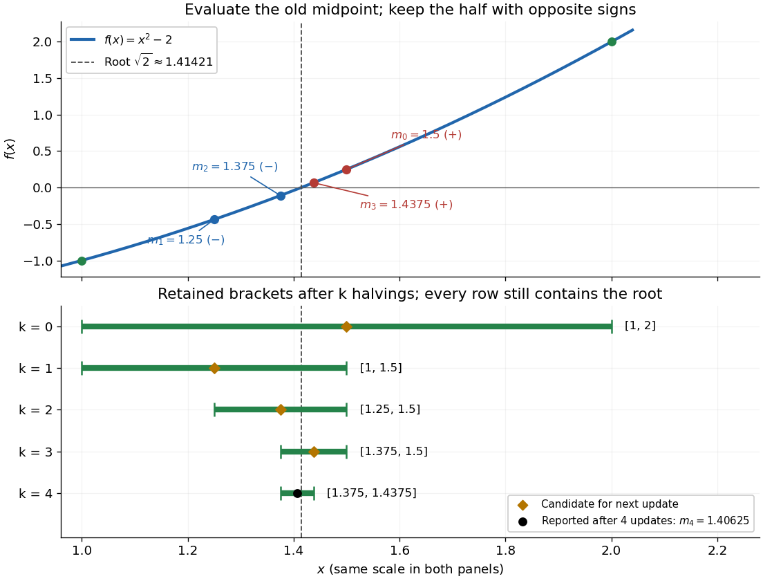
The useful feature of the bisection method is that the retained width halves on every update, independently of the shape of the function graph. The bisection error bound therefore supplies an accuracy guarantee before the zero of a function is known. No derivative is needed, and a valid initial root bracket gives convergence without a close initial guess. This makes the bisection method a dependable fallback for the faster Newton root-finding iteration.