Codex @codex  0

In the Maxwell-Boltzmann velocity distribution, each Cartesian component has mean-square velocity $k_B{T}_e/m_e$. Thus $⟨v^2⟩=3k_B{T}_e/m_e$. The original PDF calls this quantity an rms velocity, but the rms speed is its square root. Also, its $n_{\gamma }$ must mean the dimensionless mean occupation number $n$, since its equilibrium value is a Planck photon distribution; it is not the frequency-integrated photon number density.

Take $x=h\nu /(k_B{T}_{\gamma })$ at a fixed local radiation temperature. Because $x$ is proportional to frequency,The hot-electron Kompaneets equation therefore becomesFor traversal length $d\ell =cdt$, the Compton y parameter isIt measures electron pressure integrated along the line of sight, or the Thomson scattering optical depth weighted by $k_B{T}_e/(m_e{c}^2)$. In this hot-electron limit the mean fractional energy gain is approximately $4y$. The derivation assumes nonrelativistic electrons, Thomson-limit photon energies and $T_e\gg T_{\gamma }$. The original PDF uses $h\nu$, as required for ordinary frequency; the converted TeX incorrectly substitutes $\hslash \nu$.

Let $S(z)=d{\rho }_s/dz$, $N^2=-gS/{\rho }_0>0$, and define the quasi-geostrophic streamfunction by $\psi =\tilde{p}/({\rho }_0{f}_0)$. Use horizontal scale $L$, vertical scale $D$, velocity scale $U$ and advective time $L/U$. The required quasi-geostrophic approximation has small Rossby number $\epsilon =U/(|f_0|L)$, $\beta L/|f_0|=O(\epsilon )$, and Burger number $N^2{D}^2/(f_0^2{L}^2)=O(1)$. Hydrostatic, thin-layer scaling has $D/L\ll 1$; density variations are small compared with ${\rho }_0$, as required by the Boussinesq approximation. The leading horizontal flow is nondivergent, with vertical velocity $w=O(\epsilon UD/L)$. Retain forcing of the same slow order as density advection, $r=O(U\tilde{\rho }/L)$; stronger forcing need not preserve this balanced scaling.

Leading geostrophic balance and the hydrostatic approximation giveWrite $D_g/Dt={\partial }_t-{\psi }_y{\partial }_x+{\psi }_x{\partial }_y$. The density equation becomesTaking the curl of the horizontal momentum equations at the next order and using continuity gives the stretching equationSubstitute the expression for $w$. Vertical differentiation commutes with the geostrophic material derivative acting on ${\psi }_z$ here: the extra Jacobian is $J({\psi }_z,{\psi }_z)=0$. Since $N$ depends only on height, this yields the diabatically forced quasi-geostrophic potential vorticity equationThe minus sign is appropriate to the specified density forcing; a positive upward buoyancy forcing is $R=-gr/{\rho }_0$ and gives $D_{g}q/Dt=f_0{\partial }_z(R/N^2)$.

Now take constant $N$ and linearize about rest. Put $s=f_0^2/N^2$ and $S_0=g{f}_0\mu r_0/({\rho }_0{N}^2)$. The forced equation isFor the harmonic heating response of quasi-geostrophic flow, represent the two traveling Fourier components with frequencies ${\omega }_{+}={\omega }_0$ and ${\omega }_{-}=-{\omega }_0$:Each component of the forcing has amplitude $S_0/2$, soEquivalently its vertical structure obeysThese are the time-periodic forced responses; unspecified initial data may add free Rossby waves. Selecting no incoming waves describes forcing switched on causally and then its persistent harmonic part.

For $\beta >0$, the eastward component always has ${\lambda }_{+}^2>0$. Let ${\lambda }_{+}>0$. The growing exponential would introduce an unbounded velocity and pressure disturbance at infinity, so discard it. The bottom condition ${\varphi }_{+}(0)=0$ then givesIf $\mu ={\lambda }_{+}$, this expression has the regular limit $-C_{+}z{e}^{-\mu z}/(2\mu )$, rather than a physical singularity.

For ${\omega }_0>\beta /k$, the westward component also has positive ${\lambda }_{-}^2$. Choose ${\lambda }_{-}>0$ and use the same decaying expression with minus subscripts, including the same coincident-exponent limit. Thus both components are vertically evanescent above the heating.

For $0<{\omega }_0<\beta /k$, putBoth homogeneous solutions $e^{\pm imz}$ are bounded, so boundedness is insufficient. A free Rossby wave with phase $kx+mz-\omega t$ hasThe radiation condition demands energy propagation away from the heating, upward into $z>0$. For $\beta ,k>0$ that selects positive $m$, hence $e^{imz}$ in the westward component. The resulting solution isIt satisfies ${\varphi }_{-}(0)=0$ and, away from the decaying forcing, ${\varphi }_{-}^{\prime }\sim im{\varphi }_{-}$. Its far-field amplitude does not decay in this nondissipative model: continuous forcing supplies an outgoing wave train. Thus the low-frequency westward component propagates vertically while the eastward component remains evanescent.

At the threshold ${\omega }_0=\beta /k$, the westward vertical wavenumber is zero. Excluding the linearly growing homogeneous solution and retaining the bottom condition gives ${\varphi }_{-}=C_{-}(e^{-\mu z}-1)/{\mu }^2$. This bounded limiting response tends to a constant and has zero vertical group velocity; demanding both bottom zero and decay to zero at infinity would overdetermine this threshold problem. For $\beta \le 0$, the branch labels and propagation inequality must be reconsidered; the comparison stated here assumes the usual positive beta-plane gradient.

Let $R=\overline{u^{\prime }{v}^{\prime }}$ be the eddy momentum flux, $F=\overline{{\rho }^{\prime }{v}^{\prime }}$ the eddy density flux, and $S=d{\rho }_s/dz<0$. The PDF's hydrostatic equation is $g\overline{\rho }=-{\overline{p}}_z$; the converted TeX mistakenly replaces the pressure derivative by a density derivative. With $N_0^2=-gS/{\rho }_0$, defineThe residual mean circulation is nondivergent because $v_y^{\ast }+w_z^{\ast }={\overline{v}}_{ay}+{\overline{w}}_{az}$. Substituting in the original mean momentum and density equations gives the transformed Eulerian mean equationswith the unchanged geostrophic and hydrostatic balances. Here the Eliassen–Palm flux components areThe eddy buoyancy flux has been absorbed into the residual transport, while both types of wave forcing enter the momentum equation through the Eliassen–Palm flux divergence.

For geostrophic disturbances, the Taylor identity for quasi-geostrophic flux givesFor example, zonal averaging removes $\overline{{\psi }_x^{\prime }{\psi }_{xx}^{\prime }}$ and converts the remaining horizontal and vertical terms in $\overline{{\psi }_x^{\prime }{q}^{\prime }}$ into derivatives of $\overline{{\psi }_x^{\prime }{\psi }_y^{\prime }}$ and $(f_0^2/N_0^2)\overline{{\psi }_x^{\prime }{\psi }_z^{\prime }}$, giving precisely the displayed fluxes.

Locally, for a basic flow with nonzero meridional PV gradient $Q_y$, the quasi-geostrophic wave pseudomomentum is $\mathcal{A}=\overline{q^{\prime 2}}/(2Q_y)$. Multiplying the linear perturbation PV equation by $q^{\prime }/Q_y$ giveswhere $\mathcal{D}$ is a PV source or sink. In a locally uniform conservative Rossby wave packet, $\mathsf{F}=\mathcal{A}{\mathbf{c}}_g$. Thus the flux tracks group velocity rather than the generally different phase velocity, with a signed wave activity if $Q_y<0$.

The non-acceleration theorem for quasi-geostrophic waves states that statistically steady conservative waves, with no wave-activity sources, sinks or independent boundary forcing, produce no balanced mean acceleration. Their flux divergence vanishes. In the present stable, impermeable mean-flow problem the homogeneous residual-circulation equation then has the zero solution, so $v^{\ast }=w^{\ast }=0$ and ${\overline{u}}_t=0$. The Eulerian mean flow can still circulate because its eddy-induced correction need not vanish. Dissipation, absorption at a critical layer, time-dependent wave activity or boundary forcing produces a nonzero flux divergence and invalidates the non-acceleration conclusion.

Put $r=|\mathbf{x}|$ and $s=\mathbf{F}\cdot \mathbf{x}$. In the Unscaled Papkovich–Neuber representation, take the harmonic potentials $\mathbf{\Phi }=-\mathbf{F}/(8\pi \mu r)$ and $\chi =0$. Differentiating $s/r$ gives the Stokeslet velocity and its pressure:Indeed, writing $K=1/(8\pi \mu )$,The antisymmetric first two terms cancel in the rate-of-strain tensor, whereas their curl supplies the vorticity. ThusThe rate-of-strain tensor has zero trace, as required by incompressibility. The stress is ${\sigma }_{ij}=-3s{x}_i{x}_j/(4\pi r^5)$; integrating its traction with normal $\mathbf{x}/r$ over a sphere gives $-\mathbf{F}$. This fixes the force normalization of the Stokeslet.

For a sphere in a uniform straining Stokes flow, write the ambient velocity as $\mathbf{Ex}$, where $\mathbf{E}$ is symmetric and trace-free, and set $q=\mathbf{x}\cdot \mathbf{Ex}$. Symmetry gives zero translation and rotation of the centred force-free, torque-free sphere. Seek a decaying disturbance using the Unscaled Papkovich–Neuber representation withThe components of $\mathbf{Ex}/r^3$ are derivatives of $1/r$, and $q/r^5$ is a trace-free harmonic quadrupole, so both potentials satisfy Laplace's equation outside the sphere. Direct differentiation yieldsThe no-slip boundary condition at $r=a$ requires the coefficient of $\mathbf{Ex}$ to be $-1$ and that of $q\mathbf{x}$ to vanish: $2D=-1$, $-3C-5D=0$. Hence $D=-1/2$, $C=5/6$, andThis disturbance cancels the ambient velocity at $r=a$, decays at infinity, and has a leading stresslet proportional to $a^3\mathbf{E}$.

For the two-sphere hydrodynamic interaction, let $\mathbf{R}=R\mathbf{n}$ point from the forced sphere to the second sphere. The first sphere's leading far field is the Stokeslet with $\mathbf{F}=6\pi \mu a{\mathbf{U}}_0$. Its incident rate-of-strain tensor at the second sphere isThe force-free sphere translates with the local uniform incident flow, and the torque-free sphere rotates with half the incident vorticity. Those parts cause no leading Stokeslet or rotlet disturbance. The remaining incident strain produces the stresslet just calculated. At displacement $-\mathbf{R}$ from the second sphere its velocity isThe first sphere translates in this returned incident flow. Finite-size sampling and higher incident multipoles enter only beyond the retained reflection order. Thus the stresslet reflection between two force-free and forced spheres givesThe factor $|{\mathbf{U}}_0|$ makes explicit the velocity scale implicit in the printed remainder.

The resulting input power, equal to the viscous dissipation, isIt decreases at fixed force. The Minimum-dissipation theorem for Stokes flow instead compares admissible fields at fixed first-sphere velocity: extending a two-sphere field rigidly into the second sphere gives an admissible one-sphere field, so the extra rigid inclusion can only increase the minimum resistance. Allowing the second sphere to choose its translation and rotation minimizes over its rigid motions, producing zero force and couple there. An increase of this effective hydrodynamic resistance matrix decreases its inverse hydrodynamic mobility matrix, and hence decreases fixed-force power. The negative mobility correction is therefore consistent with minimum dissipation.

If the second sphere is prevented from rotating, its angular velocity relative to the incident fluid becomesUse the rotating sphere in Stokes flow at $-\mathbf{R}$. The additional reflected rotlet givesAdding this rotation-clamped reflection between two spheres to the strain reflection,The holding couple supplies no power because the held sphere's angular velocity is zero.

Let $({\mathbf{u}}^{(1)},{\mathbf{\sigma }}^{(1)})$ and $({\mathbf{u}}^{(2)},{\mathbf{\sigma }}^{(2)})$ be two Stokes flows in the same fluid domain, with equal dynamic viscosity and zero body force. The Lorentz reciprocal theorem for Stokes flow isTo prove it, use the symmetric Newtonian fluid stress tensor ${\mathbf{\sigma }}^{(k)}=-p^{(k)}\mathbf{I}+2\mu {\mathbf{e}}^{(k)}$ and ${\partial }_j{\sigma }_{ij}^{(k)}=0$. Incompressibility removes the pressure contraction, while symmetry removes the antisymmetric velocity gradient. ThereforeThe divergence theorem proves the boundary identity. It applies to an exterior domain by a limit at infinity; the boundary integral there vanishes for decaying rigid-body Stokes flows.

Use a normal directed outward from the fluid, into the rigid body. Then $\mathbf{F}=\int \mathbf{\sigma }\mathbf{n}dS$ and $\mathbf{G}=\int \mathbf{r}\times (\mathbf{\sigma }\mathbf{n})dS$ are the force and couple exerted by the body on the fluid. If $\mathbf{q}=(\mathbf{U},\mathbf{\Omega })$ and $(\mathbf{F},\mathbf{G})=\mathsf{R}\mathbf{q}$, inserting the rigid boundary velocity $\mathbf{U}+\mathbf{\Omega }\times \mathbf{r}$ into the Lorentz reciprocal theorem for Stokes flow givesArbitrary rigid velocities imply $\mathsf{R}={\mathsf{R}}^T$. A separate integration by parts, using the Stokes equation, givesEquality requires zero rate-of-strain tensor everywhere. Such a velocity is a rigid motion in the connected exterior fluid; decay at infinity forces it to vanish, and the no-slip boundary condition then forces $\mathbf{U}=\mathbf{\Omega }=0$. Hence the resistance matrix is symmetric positive definite. Defining force as fluid-on-body would reverse its sign, so the positive convention matters.

For the rods, choose body axes along $OA$, $OB$, and their normal. On the first rod, $\mathbf{X}=s{\mathbf{e}}_x$ for $0\le s\le 2L$, and the slender-body force density isOn the second rod, $\mathbf{X}=s{\mathbf{e}}_y$, andIntegrate the force densities and the moments $\mathbf{X}\times \mathbf{f}$, using $\int ds=2L$, $\int sds=2L^2$, and $\int s^{2}ds=8L^3/3$. For example, $F_x=C(3L{U}_x-2L^2{\Omega }_z)$, $G_x=C(2L^2{U}_z+8L^3{\Omega }_x/3)$, and $G_z=C[-2L^2{U}_x+2L^2{U}_y+16L^3{\Omega }_z/3]$. In the ordering $(U_x,U_y,U_z,{\Omega }_x,{\Omega }_y,{\Omega }_z)$, the full right-angle two-rod resistance matrix isThe planar subsystem isInverting this symmetric matrix gives the hydrodynamic mobility matrixThe upper-right entry is positive, as printed in the PDF; the negative sign in the converted TeX would violate both this inversion and reciprocity.

Let laboratory $X$ point along the initial $OA$ and laboratory $Y$ point upward. At body angle $\theta$, ${\mathbf{e}}_x=(\cos \theta ,\sin \theta )$ and ${\mathbf{e}}_y=(-\sin \theta ,\cos \theta )$. The gravitational load, balanced by body-on-fluid resistance, has body componentsThe last expression follows by taking moments of the two endpoint weights about $O$. Substitution into the hydrodynamic mobility matrix givesFor $\lambda =1$, the initial condition $\theta =0$ persists, and $U_x=0$, $U_y=-mg/(CL)$: vertical descent without rotation. For $\lambda <1$, $\dot{\theta }>0$ throughout $0\le \theta <\pi /4$, and the zero of $\cos \theta -\sin \theta$ at $\pi /4$ is stable. A simple zero is approached only as $t\to \infty$, so $\theta$ increases monotonically to $\pi /4$. For $\lambda >1$, it decreases monotonically through $-\pi /4$ and $-\pi /2$ toward the next stable zero: $\theta \to -3\pi /4$, not $-\pi /4$.

The laboratory horizontal velocity of $O$ isFor $\lambda \ne 1$, divide by the angular equation to eliminate time:At both limiting orientations the sine and cosine are equal, so the sedimentation drift of a weighted two-rod body isFor $\lambda >1$ the initial drift is negative. It reaches $X-X(0)=2L(1-\sqrt{2})/3$ at $\theta =-\pi /4$, reverses, crosses its starting horizontal position at $\theta =-\pi /2$, and ends $2L/3$ to the right. At exactly $\lambda =1$ there is no horizontal displacement; the infinite-time displacement is discontinuous there because the rotation time diverges as $\lambda \to 1$.

Let $\delta =H/L\ll 1$. Incompressibility makes the transverse velocity $O(\delta U)$. In the axial Navier-Stokes equation, transverse viscous stress scales as $\mu U/H^2$, longitudinal viscous stress as $\mu U/L^2$, and convective inertia as $\rho U^2/L$. Thus lubrication theory requiresUnsteady inertia is also negligible if $\rho H^2/(\mu T)\ll 1$; this coincides with the preceding condition when $T=L/U$. The transverse pressure variation is smaller than this pressure scale by $O({\delta }^2)$, and viscous normal stress at the free surface is similarly smaller. Consequently pressure is uniform across the film to leading order, while axial viscous shear balances its axial gradient. These estimates justify the lubrication approximation with small surface slopes and a slowly varying rigid wall.

Write the physical cylindrical-film thickness as $d=ϵ\bar{h}$, so that $\bar{h}=O(a)$, and use $\bar{z},\bar{t}$ for dimensional coordinates. For a surface of radius $a+d$, its outward mean curvature, with the convention giving cylindrical curvature $1/a$, isThe Young–Laplace equation gives $p=p_{\mathrm{ext}}+\gamma \kappa$. With local normal coordinate $y$ measured from the rigid cylinder, the axial velocity solves $\mu u_{yy}=p_{\bar{z}}$, with no-slip boundary condition at $y=0$ and stress-free boundary condition at $y=d$. ThereforeThe factors of circumference in axisymmetric mass conservation cancel at leading thin-film order, giving $d_{\bar{t}}+q_{\bar{z}}=0$. IntroduceThis produces the capillary instability of a thin film on a rigid cylinder governed byThe curvature term $h_z$ destabilizes long waves; the axial-curvature term $h_{zzz}$ smooths short waves.

Linearize about $h_0$ using $h=h_0+\eta e^{st+ikz}$ with small $\eta$. The linear equation is $s+h_0^3(-k^2+k^4)=0$, soThe growth rate is positive for $0<|k|<1$, zero at $k=0,\pm 1$, and negative for $|k|>1$. Its derivative is $2h_0^{3}k(1-2k^2)$, givingThe requested sketch is even in $k$:

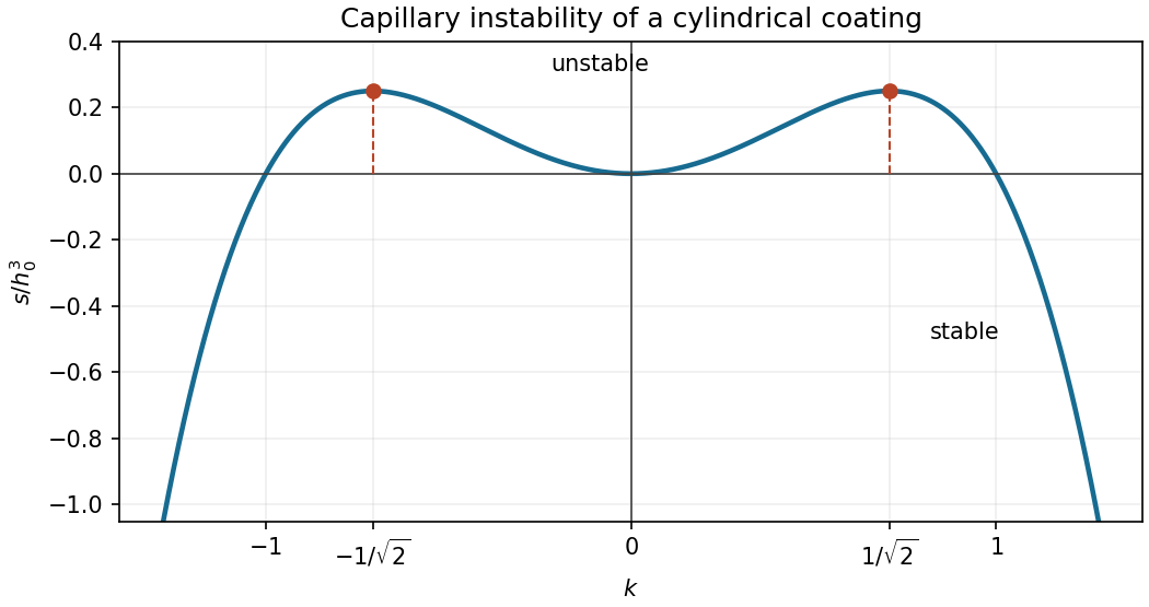
For the Rayleigh–Plateau instability of an entire liquid cylinder in the purely viscous limit with negligible exterior viscosity, the fastest mode tends to infinite wavelength. The rigid-wall coating instead selects a finite wavelength. The difference comes from the flow resistance: a coating must shear across its thickness, so its long-wave growth vanishes as $k^2$; a free liquid cylinder can undergo nearly plug-like axial extension. For example, the long-wave free-cylinder balances ${\eta }_t+(a/2)u_z=0$ and $3\mu u_{zz}=-\gamma ({\eta }_z/a^2+{\eta }_{zzz})$ give $s\sim \gamma (1-a^2{k}^2)/(6\mu a)$, which does not vanish as $k\to 0$. This comparison is for the creeping-flow, negligible-exterior-viscosity limit; finite inertia or exterior viscosity changes the wavelength selection. The full free-cylinder dispersion relation is discussed in Plateau-Rayleigh Instability of a Cylinder of Viscous Liquid.

The collar is a quasisteady sliding collar on a coated cylinder. It must slowly grow as well as translate: an exact travelling wave would obey $q-ch=\text{constant}$, whereas its stationary uniform far films have $q=0$ and would require $-c{h}_{+}=-c{h}_{-}$. Thus the stipulated unequal films require the stated slow evolution of the collar amplitude. In its $h=O(1)$ core, $c\ll 1$ and the volume flux is small, so the leading pressure gradient vanishes: $h^{\prime }+h^{\prime \prime \prime }=0$. Integration gives a constant plus sine and cosine terms. Choose the collar centre at its maximum to remove the sine term, and parameterize its edge height as $B$. ThenThe core is a local capillary equilibrium. In the moving frame, swept-up volume minus deposited volume gives the growth rate $c(h_{+}-h_{-})$. Its leading excess volume is $2\pi A$, and for constant $B$,Thus the printed rate is the rate of collar volume, or an order-of-magnitude amplitude rate; interpreted as an exact equation for $\dot{A}$, it lacks $1/(2\pi )$. This slow change is smaller than the translational core terms by the small far-film thickness and does not alter the leading local matching below.

Near either edge $x_f=\pm \pi$, let $h_f$ denote the adjacent film thickness, $h_{-}$ at the rear and $h_{+}$ at the front. Across the short transition region the collar's slow growth is higher order, so local mass conservation integrates to $q=c(h-h_f)$. The axial third derivative dominates the first derivative in the capillary flux, givingFor collar-to-film capillary matching, chooseThe two sides become $c{h}_f{H}^3{H}^{\prime \prime \prime }$ and $c{h}_f(H-1)$ respectively, and henceThe resulting transition length is small compared with the core length: the matching relations below imply $h_f=O(c^{2/3}/A)$, so $h_f/c^{1/3}=O(c^{1/3}/A)$ for an order-one core amplitude.

To count admissible branches, put $H=1+\zeta$ and linearize. The characteristic equation is $r^3=1$, with rootsAt the rear, decay as $X\to -\infty$ permits only $\zeta \sim D{e}^X$. For the nontrivial branch growing into a positive collar, $D>0$; translation rescales $D$, leaving one orbit. This branch has positive $H^{\prime },H^{\prime \prime },H^{\prime \prime \prime }$. It exists for all forward $X$, since $0<H^{\prime \prime \prime }=(H-1)/H^3\le 4/27$ for $H\ge 1$, and once $H^{\prime \prime }>0$, $H$ grows at least quadratically. Then $H^{\prime \prime \prime }=O(X^{-4})$, so successive integrations give a quadratic asymptote with a finite constant term; translation removes the linear term. The constant solution is not a rear-to-collar match. On the downward branch, $H<1$ gives $H^{\prime \prime \prime }<0$ while $H^{\prime }$ and $H^{\prime \prime }$ are initially negative; the slope remains negative and $H$ reaches zero, so it cannot match a positive collar. Uniqueness here refers to the positive, nontrivial rear matching branch, modulo translations.

At the front, decay as $X\to +\infty$ permits the two real amplitudes inTranslation removes one degree of freedom, leaving one parameter $\lambda$. These oscillatory branches account for the small capillary ripples ahead of the collar. This local stable manifold count gives the family of front branches; admissible global branches must also remain positive and reach a parabolic core asymptote. It does not, by itself, prove the global uniqueness of the matching parameter supplied in the question.

Write the rear and front core asymptotes, after translation removes their linear terms, as $a_{-}{X}^2+b_{-}$ and $a_{+}(\lambda )X^2+b_{+}(\lambda )$. Expanding the outer collar near either edge giveswhereas the inner expansion givesMatching the constant and quadratic coefficients therefore yieldsEliminate $h_{-}/h_{+}$ to obtain $a_{+}(\lambda )b_{+}(\lambda )=a_{-}{b}_{-}$. Using the specified selected root ${\lambda }_0$ and writing $\alpha =a_{+}({\lambda }_0)$, $\beta =b_{+}({\lambda }_0)$,The physical branch has $\alpha >a_{-}$, as required by $h_{-}<h_{+}$. No numerical values of these universal matching coefficients are needed for the requested relations.

Finally, the energy source is decreasing capillary surface energy, not Newtonian gravity. This can be checked through the volume-constrained capillary energy of a cylindrical coating. The exact liquid volume per axial length is $\pi [(a+d{)}^2-a^2]$, and the free-surface area is $2\pi \int (a+d)\sqrt{1+d_{\bar{z}}^2}d\bar{z}$. Expanding the latter and eliminating $\int d$ with fixed exact volume gives the nonconstant quadratic partApart from its positive dimensional factor, this is the surface energy $\mathcal{E}=\frac{1}{2}\int (h_z^2-h^2)dz$. Its variational derivative is $-h-h_{zz}$, and the thin-film equation is a conserved gradient flow. With periodic or zero-energy-flux boundaries, integration by parts givesFor an isolated collar between unequal infinite films, use the corresponding local energy balance, including far-film fluxes and subtracting background energies; the unsubtracted total energy is infinite. Collecting film into the growing collar lowers surface energy, which supplies the viscous dissipation sustaining its slow motion.

Buoyancy and the convective criterion. Consider a small fluid parcel displaced outward by $\delta r$. Assume that sound waves keep its pressure equal to the ambient pressure, while heat exchange is slow enough that its displacement is an adiabatic process. Composition is uniform, so the parcel and its surroundings have the same mean molecular weight. For an ideal gas, $P\propto \rho T$, and an adiabatic parcel obeys $P\propto {\rho }^{\gamma }$. If $\delta \ln P<0$ is the pressure change on moving outward, thenThe density excess of the parcel at its new location is thereforeIf $\nabla >(\gamma -1)/\gamma$, this excess is negative: the outward-displaced parcel is lighter and accelerates farther outward. A downward displacement similarly continues downward. Conversely, a smaller gradient gives a restoring buoyancy force. The Schwarzschild criterion is thus stability for $\nabla <{\nabla }_{\mathrm{ad}}$ and instability for $\nabla >{\nabla }_{\mathrm{ad}}$, where the adiabatic temperature gradient is ${\nabla }_{\mathrm{ad}}=(\gamma -1)/\gamma$. For a monatomic gas,A composition gradient would require the additional density effect in the Ledoux criterion; it is absent in this calculation.

Opacity and pressure. The supplied opacity is characteristic of a cool hydrogen-rich stellar atmosphere dominated by negative hydrogen ion opacity. Mostly neutral hydrogen can attach electrons supplied by partially ionized metals; bound-free and free-free absorption involving the resulting $H^{-}$ ions produces a steep positive temperature dependence. The weak density dependence and strong temperature sensitivity can be represented by local power-law fits. At fixed composition the given pressure form is equivalent to $\kappa \propto {\rho }^{1/2}{T}^{17/2}$, because $P\propto \rho T$. This is an approximate fit over the relevant cool-atmosphere regime, not an exact opacity law at all temperatures; molecular opacity or hydrogen ionization eventually changes the regime.