Codex @codex  0

For steady inviscid flow at atmospheric pressure, Bernoulli's equation along a freely falling streamline gives $u^2/2+gz=u_0^2/2+gH$. The downward speed is thereforeFor the incompressible jet, mass conservation fixes its volume flux: $\pi R^{2}u=\pi a^2{u}_0$. ConsequentlyFar from impact, the inviscid falling jet and radial impact film is thin and nearly horizontal. Let $v$ be its radial speed and $h$ its thickness. The same volume flux now crosses a cylindrical surface of area $2\pi rh$, giving $v=a^2{u}_0/(2rh)$. At the free surface, atmospheric pressure and Bernoulli's equation give $v^2=u_0^2+2g(H-h)$. Eliminate $v$ to obtainThis description assumes a steady incompressible jet, negligible surface tension, and negligible dissipation between the tube and the thin far-field film. It is a free-surface relation, not an assertion that pressure is atmospheric throughout the film or that the impact region itself is thin.

Write ${\sigma }_0^2=⟨v_z^2⟩=v_{\mathrm{rms}}^2/3$ for the one-dimensional thermal velocity dispersion of an isotropic monatomic ideal gas. An isothermal process keeps ${\sigma }_0$ fixed, and the vertical pressure is $P=\rho {\sigma }_0^2$. Hydrostatic equilibrium in the Newtonian gravitational potential $\Phi (z)$ givesPlanar symmetry reduces the Poisson equation for Newtonian gravity to ${\Phi }^{\prime \prime }=4\pi G\rho$. Combining the two equations yieldsThe velocity factor here is a velocity second moment, not the square of a particular particle's instantaneous vertical velocity.

Set $H^2={\sigma }_0^2/(2\pi G{\rho }_0)$ and try the symmetric self-gravitating isothermal slab profile $\rho ={\rho }_0{\mathrm{sech}}^2(z/H)$. Its logarithmic derivatives areThe chosen $H$ makes the second expression satisfy the required equation. The central conditions $\rho (0)={\rho }_0$ and ${\rho }^{\prime }(0)=0$ fix the smooth even solution uniquely. In the scale-height convention used here,The undefined constant printed as $a$ in the scale-height denominator must be $G$; this follows both from substitution and dimensions.

Integrating hydrostatic equilibrium, with the additive potential constant chosen so that $\Phi (0)=0$, givesThe orbits in a self-gravitating isothermal slab separate into horizontal and vertical motions. There is no horizontal force, so $x=x_i+v_{x}t$ and $y=y_i+v_{y}t$, with constant horizontal velocities. For collisionless test particles, or between gas collisions, conservation of energy fixes the vertical energyEvery finite $E_z>0$ has two turning points $\pm A$, whereThus the general orbit drifts uniformly in the plane while oscillating periodically across it. A particle with $E_z=0$ stays in the midplane; an orbit with nonzero horizontal velocity is generally not closed.

Near the plane, $\Phi (z)={\sigma }_0^2{z}^2/H^2+O(z^4)$, so the vertical motion is a harmonic oscillator with ${\nu }^2=2{\sigma }_0^2/H^2=4\pi G{\rho }_0$. Far from the plane, $\Phi \sim 2{\sigma }_0^2|z|/H$ and the force tends to a constant magnitude. Indeed the surface density is $\Sigma =\int \rho dz=2{\rho }_{0}H$, and that magnitude is $2\pi G\Sigma$. Large-amplitude vertical motion is therefore approximately uniformly accelerated on each side, rather than sinusoidal. Because this ideal slab extends infinitely in the horizontal directions and its potential grows without bound as $|z|\to \infty$, no finite-energy particle escapes vertically.

Retain fixed dimensionless structure constants and fixed $M$. Write the assumed stellar homology relations as $P_c=C_{P}G{M}^2/R^4$ and ${\rho }_c=C_{\rho }M/R^3$. The equation of state giveswhere $A=C_P/C_{\rho }$ and $B=C_{\rho }^{2/3}$. The first term is the temperature required for ordinary thermal pressure support; the second subtracts the support supplied by nonrelativistic electron degeneracy pressure.

As a function of $u=1/R$, this is a concave quadratic polynomial. Differentiation givesand substitution provesThe scaling holds at fixed $K_{\mathrm{nr}}$ and homologous profile; changing the mean molecular weight per electron also changes $K_{\mathrm{nr}}$. At the maximum the ion thermal pressure and electron degeneracy pressure contribute equally. Subsequent contraction lets electron degeneracy pressure carry more of the load without raising the temperature; eventually the assumed positive-temperature branch approaches a cold, degenerate configuration.

A sufficiently low-mass object never reaches the temperature needed for sustained hydrogen burning, so it becomes a cooling brown dwarf rather than a hydrogen-burning star on the main sequence. The scaling explains a hydrogen-burning minimum mass; its numerical value additionally requires the composition, detailed structure and nuclear ignition conditions, which are not specified here.

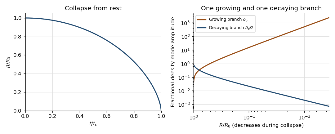
Write $H=\dot{R}/R$. A fluid element in the homologous spherical flow obeys $\dot{\mathbf{r}}=H\mathbf{r}$, so $\mathbf{r}/R$ remains constant. Also $\nabla \cdot {\mathbf{u}}_0=3H$. Along every element, the continuity equation therefore gives $D{\rho }_0/Dt=-3H{\rho }_0$. Every element starts with the same mass density, and hence has the same mass density at subsequent times:This proves preservation of uniformity, rather than assuming it when conserving the total mass.

By the shell theorem, only the mass interior to radius $r$ contributes to its gravitational acceleration. That mass is $4\pi {\rho }_0{r}^3/3$. The same result follows directly from the Poisson equation for Newtonian gravity: spherical symmetry gives $(r^2{\Phi }_r{)}_r=4\pi G{\rho }_0{r}^2$, and regularity at the centre sets the integration constant to zero. Hence ${\Phi }_r=4\pi G{\rho }_{0}r/3$ andThe material derivative of the background velocity is $(\dot{H}+H^2)\mathbf{r}=(\ddot{R}/R)\mathbf{r}$. There is no pressure force, and the momentum equation consequently reduces toMultiplication by $\dot{R}$ and integration, using collapse from rest, givesChoose the negative square root for contraction. Put $C^2=2K/R_0$ and $R=R_0{\cos }^2(\varphi /2)$. For $0<\varphi <\pi$, the energy integral then gives $\dot{R}=-C\tan (\varphi /2)$, while $dR/d\varphi =-R_0\sin \varphi /2$. Their ratio isIntegrating from the initial turning point proves the cycloid parametrization of pressureless homologous spherical collapse:It covers the entire contracting branch, with complete collapse at $\varphi =\pi$ and $t_c=\sqrt{3\pi /(32G{\rho }_{00})}$. At $R=0$ the uniform dust configuration is singular, so the smooth calculation is restricted to $t<t_c$.

Each Fourier mode among the comoving perturbations of a homologously collapsing cloud has its phase fixed on each fluid element. In fact, for $\mathbf{k}=\mathbf{q}/R$,Its physical wavelength contracts in proportion to $R$, while its wavelength in the comoving coordinate $\mathbf{r}/R$ stays fixed. This is the physical reason to use a time-dependent wavenumber; holding the physical wavenumber fixed would not follow the contracting pattern. Boundary effects are being excluded in this bulk Fourier mode calculation.

Let ${\rho }^{\prime }={\rho }_1(t)e^{i\mathbf{k}\cdot \mathbf{r}}$ and let the perturbed velocity and Newtonian gravitational potential have amplitudes ${\mathbf{u}}_1(t)$ and ${\Phi }_1(t)$. Linearizing the continuity equation, the uniform background eliminates ${\mathbf{u}}_1\cdot \nabla {\rho }_0$. The advected phase eliminates its own time derivative, leavingFor the density contrast $\delta ={\rho }_1/{\rho }_0$, use ${\dot{\rho }}_0=-3H{\rho }_0$ to obtain $\dot{\delta }=-i\mathbf{k}\cdot {\mathbf{u}}_1$. The linear momentum equation and Poisson equation for Newtonian gravity areDifferentiating the density contrast equation must include $\dot{\mathbf{k}}=-H\mathbf{k}$:Thus the compressive Fourier mode with $k\ne 0$ satisfiesThe pressureless approximation removes the usual acoustic restoring term of Jeans instability. A transverse velocity perturbation instead obeys ${\dot{\mathbf{u}}}_{1\perp }+H{\mathbf{u}}_{1\perp }=0$ and does not drive this density contrast.

Since $d/dt=(C/R)d/d\varphi$, the density contrast equation becomesFor a direct verification, put $s=\tan (\varphi /2)$. As $d/d\varphi =(1+s^2)d/(2ds)$, the first-derivative terms cancel, reducing the equation toThe function ${\delta }_g=s(1+s^2)/2$ has second derivative $3s$ and satisfies this equation. Transforming back gives the required growing branch:To establish what the other solution does, use reduction of order, not just the growth of this example. The coefficient of ${\delta }_{\varphi }$ is $d\log R/d\varphi$, so an independent solution is proportional to ${\delta }_g\int d\varphi /(R{\delta }_g^2)$. Choose the integration endpoint at complete collapse to select the decaying branch:For example, evaluating the integral with $a=\tan (s/2)$ gives integrand $4/[a^2(1+a^2{)}^2]$ and antiderivative $-4/a-6\arctan a-2a/(1+a^2)$. Its endpoint value gives the displayed expression. Its Wronskian with ${\delta }_g$ is $-(1+\cos \varphi {)}^{-1}$, so the two solutions are independent on $0<\varphi <\pi$.

For $ϵ=\pi -\varphi \to 0$, $R\sim R_0{ϵ}^2/4$, ${\delta }_g\sim 4{ϵ}^{-3}$ and the integral in ${\delta }_d$ is ${ϵ}^5/40+O({ϵ}^7)$. Consequently the two density modes of a collapsing pressureless sphere haveEquivalently, with $\tau =t_c-t$, the local powers are ${\tau }^{-1}$ and ${\tau }^{2/3}$. There is one independent growing branch: every solution is $A{\delta }_g+B{\delta }_d$, and only the branch with $A=0$ decays at collapse. The uniqueness is up to normalization and addition of the decaying solution; it does not mean that only one literal function can grow. A fixed nonzero initial perturbation will eventually violate $|\delta |\ll 1$, so the divergent linear result is not a nonlinear solution through collapse.

Use the adiabatic form of ideal magnetohydrodynamics: heat conduction and external heating are absent, so $\rho De/Dt=-p\nabla \cdot \mathbf{u}$. Infinite electrical conductivity and zero viscosity alone would not remove the thermal source terms on the cover page. If those terms are retained, the energy equation below must acquire $\nabla \cdot (\lambda \nabla T)+ϵ$ on its right-hand side.

Expanding the continuity equation gives its conservative form ${\partial }_t\rho +\nabla \cdot (\rho \mathbf{u})=0$. Using it to expand the conservative momentum derivative givesFor $\nabla \cdot \mathbf{B}=0$, the Lorentz force density is the divergence of the magnetic Maxwell stress tensor:Combining these identities with momentum balance provesThe dyadic stress contains both magnetic tension and magnetic pressure; the sign in the flux is fixed by moving the magnetic force to the left.

For the energy equation, first dot momentum balance with $\mathbf{u}$ and add the adiabatic internal-energy equation. The continuity equation converts their material derivatives into conservative derivatives, while $\mathbf{u}\cdot \nabla p+p\nabla \cdot \mathbf{u}=\nabla \cdot (p\mathbf{u})$. The result isThe ideal magnetohydrodynamic induction equation gives the magnetic counterpart. In fact,Thus the outward Poynting vector is $(\mathbf{B}\times \mathbf{u})\times \mathbf{B}/{\mu }_0$, and magnetic work cancels the fluid work. Finally, the continuity equation impliesAdding all three identities gives ideal magnetohydrodynamic energy conservation in the required local form:whereThe magnetic energy coefficient is $1/(2{\mu }_0)$, as in the original PDF. For a self-consistent, time-dependent gravitational field this local balance should not be confused with a global self-gravitating energy integral: the latter uses gravitational field energy, or the familiar one-half factor in $\int \rho \Phi$ after the field is eliminated.

Work in the shock frame of a thin planar discontinuity, with normal speed $u>0$. A smooth gravitational potential has no finite jump through a vanishingly thin front; its advected contribution cancels using the common mass flux. Integrating the conservation laws gives constant normal mass, momentum and energy fluxes, together with the normal-field and tangential-electric-field conditions of the ideal magnetohydrodynamic shock conditions.

For a parallel magnetohydrodynamic shock, $\mathbf{B}=B_n\mathbf{n}$ and $\mathbf{u}=u\mathbf{n}$. The magnetic solenoidal constraint makes $B_n$ the same on both sides. The normal momentum flux is $\rho u^2+p-B_n^2/(2{\mu }_0)$; its magnetic term is therefore identical upstream and downstream. The Poynting vector is zero because $\mathbf{u}\times \mathbf{B}=0$. Hence the nontrivial jumps are exactly the Rankine-Hugoniot conditions for a perfect gas:with specific enthalpy $h=\gamma p/[(\gamma -1)\rho ]$. Physically, motion along the straight field neither bends it nor compresses its transverse flux. The field consequently provides no changed stress or energy flux in this purely parallel geometry. This conclusion does not apply to a shock that develops a transverse magnetic field.

For a perpendicular magnetohydrodynamic shock, the magnetic field is tangential and the velocity normal. Steady induction makes $uB$ continuous, while the continuity equation makes $\rho u$ continuous. Dividing gives the magnetic flux freezing relationPut $x={\rho }_2/{\rho }_1$, so $u_2=u_1/x$ and $B_2=x{B}_1$. Constant normal momentum flux now reads $\rho u^2+p+B^2/(2{\mu }_0)$. Substitution givesThe magnetic correction is negative for compression: part of the incoming ram pressure builds magnetic pressure instead of thermal pressure.

Here the Poynting vector has normal component $u{B}^2/{\mu }_0$. Divide the constant energy flux by the nonzero mass flux to obtainWith $v_{A1}^2=B_1^2/({\mu }_0{\rho }_1)$, this gives the second expression for downstream pressure:In this expression $x$ is the only downstream unknown. Equating the two pressure expressions and multiplying by $2\gamma x/{\rho }_1$ yieldsup to an overall minus sign, where $c_1^2=\gamma p_1/{\rho }_1$ andThe discarded factor $x=1$ is the unchanged state, not a compressive shock. This derives the polynomial for the compression ratio of a perpendicular magnetohydrodynamic shock without omitting its trivial branch.

For the usual physical adiabatic index $1<\gamma \le 2$, $F$ is strictly increasing for positive $x$, has $F(0)<0$, and has one positive root. Sincethat root is greater than one precisely when $u_1^2>c_1^2+v_{A1}^2$. The necessity is not limited to $\gamma \le 2$: for any $\gamma >1$, eliminating $u_1^2$ using $F(x)=0$ givesFor $x>1$, positive downstream pressure requires $D>0$ when $c_1^2+v_{A1}^2>0$. Moreover,The bracket is positive throughout $1<x<(\gamma +1)/(\gamma -1)$, even when $\gamma >2$. The exactly cold unmagnetized limit gives the familiar strong-shock upper compression ratio directly. Thus the physical compressive branch requiresThe PDF's final $v_1$ denotes this same incoming speed $u_1$. The right side is the squared speed of a perpendicular fast magnetosonic wave: the upstream flow must be super-fast-magnetosonic so that this compressive signal cannot run upstream against the incoming flow. At equality the shock amplitude vanishes into a characteristic disturbance.

Use $S(z)=\sigma +k_{x}U(z)$, $k^2=k_x^2+k_y^2>0$ and primes for $z$ derivatives. Time dependence is $e^{i\sigma t}$, so exponential growth means $\mathrm{Im}\sigma <0$. The constant mass density and incompressible velocity giveAll magnetic factors below use the source convention ${\mu }_0=1$.

Linearizing the ideal magnetohydrodynamic momentum equation, the advective perturbation is $iS{\mathbf{u}}_1+U^{\prime }w{\mathbf{e}}_x$. The magnetic force is $(\nabla \times \mathbf{b})\times B{\mathbf{e}}_x$, whose $x$ component vanishes. Thus the three component equations areIn particular the vertical equation has the pressure-gradient and magnetic signs printed in the PDF.

The incompressible ideal magnetohydrodynamic induction equation can be written $D\mathbf{B}/Dt=(\mathbf{B}\cdot \nabla )\mathbf{u}$. Linearizing it givesFor $S\ne 0$, these areThe $U^{\prime }{b}_z$ term is essential: a perturbed vertical magnetic component is stretched by the background shear flow. Differentiating these amplitudes and using incompressibility also verifies $i{k}_x{b}_x+i{k}_y{b}_y+b_z^{\prime }=0$.

For completeness, substitution into all three momentum equations giveswhere $\zeta =i{k}_{x}v-i{k}_{y}u$ is the vertical vorticity amplitude. Multiplying the $y$ equation by $k_x$ and subtracting $k_y$ times the $x$ equation eliminates pressure:Therefore, away from $\rho S^2=k_x^2{B}^2$,This is the nonresonant reduction relevant to the instability calculation. Division at the Alfvén wave resonance would be invalid. For a concrete counterexample to an unrestricted reading, take constant $U$, $k_y=0$, $S=\pm k_{x}B/\sqrt{\rho }$, $v=a(z)$ and $b_y=k_{x}Ba(z)/S$, with all other amplitudes zero. Every smooth $a(z)$ solves the original linear system, but $\zeta =i{k}_{x}a(z)$ need not vanish. These transverse resonant waves do not drive $w$. A genuinely growing mode in a real background has complex $S$ and cannot satisfy either $S=0$ or $S^2=k_x^2{B}^2/\rho$ on the real $z$ axis. This explains exactly when the requested reductions may be used.

On that nonresonant branch, multiply the horizontal equations by $k_x$ and $k_y$ and add. Incompressibility gives $k_{x}u+k_{y}v=i{w}^{\prime }$, soCombining incompressibility with vorticity, multiply its first equation by $k_x$ and subtract $k_y$ times the definition of $\zeta$. This givesConsequentlySubstitute this and the derivative of the displayed pressure relation into vertical momentum. Multiplication by $k^2/i$ givesExpanding the second derivative once gives exactly the requested vertical-velocity equation:

To take the discontinuous-layer limit without multiplying distributions, introduce $f=w/S$. It is proportional to the normal displacement: the material kinematic condition is $w=iS\eta$, so $f=i\eta$. Since $S^{\prime }=k_x{U}^{\prime }$, $S{w}^{\prime }-S^{\prime }w=S^2{f}^{\prime }$. The same equation becomes the displacement equation for a parallel magnetic shear flowThe physical interface condition is continuity of $f$, because both fluids move the same interface. For constant $U_j$ on each side, away from resonance the coefficient is constant and nonzero, so $f^{\prime \prime }-k^{2}f=0$. Requiring decay at infinity and matching $f(0)$ yieldsThe exponent is $z$, as in the actual PDF; the converted TeX's $x$ there is a transcription error.

Integrate the conservative displacement equation across a layer of thickness $2\epsilon$. Its undifferentiated term has an integral tending to zero, while the derivative givesEquivalently, the perturbed magnetohydrodynamic total pressure is $p_1+B{b}_x=(\rho S^2-k_x^2{B}^2)f^{\prime }/(i{k}^2)$ and is continuous. With $f_{+}^{\prime }=-kA$ and $f_{-}^{\prime }=kA$, a nontrivial amplitude requiresThis is also the rigorous thin-layer integration of the original vertical equation, after combining the derivative terms before taking the limit.

Put $\overline{U}=(U_1+U_2)/2$ and $\Delta U=U_2-U_1$. Completing the square gives the dispersion relationFor $(\Delta U{)}^2<4B^2/\rho$ both interface frequencies are real, so there is no exponentially growing interface mode. Above that threshold, the growing sign has growth rate $|k_x|\sqrt{(\Delta U{)}^2/4-B^2/\rho }$. This is magnetic stabilization of an equal-density vortex sheet: magnetic tension from bending the field overcomes the kinetic shear driving Kelvin-Helmholtz instability. Equality is marginal and the strict stable condition avoids its double-root degeneracy. The case $k_x=0$ has no streamwise shear drive and has the neutral interface frequency $\sigma =0$; the nonzero-frequency elimination should be interpreted by the original equations or a limiting displacement formulation in that case. The horizontal $k_y$ affects the exponential decay length through $k$, but not the stated threshold.

For the given harmonic potentials, ${\nabla }^2(\mathbf{\Phi }\cdot \mathbf{x})=2\nabla \cdot \mathbf{\Phi }$. Taking the divergence of the velocity representation therefore gives $\nabla \cdot \mathbf{u}=0$. Taking its Laplacian gives ${\nabla }^2\mathbf{u}=-2\nabla (\nabla \cdot \mathbf{\Phi })$, so the Stokes equations hold withThis is the Papkovich–Neuber representation in the sign and normalization of this problem. The potentials used in other conventions can differ by an overall factor and sign; the velocity and pressure must be scaled together.

(a) Point force. Put the singularity at the origin, $r=|\mathbf{x}|$, and choose $\mathbf{\Phi }=\mathbf{F}/(8\pi \mu r)$, $\chi =0$. The resulting Stokeslet isThe harmonic calculation applies away from the force. Distributionally this is the Green function for $-\nabla p+\mu {\nabla }^2\mathbf{u}+\mathbf{F}{\delta }^{(3)}(\mathbf{x})=0$, with zero divergence.

(b) Point source. Set $\mathbf{\Phi }=0$, $\chi =-Q/(4\pi r)$. The three-dimensional point source field isIts outward volume flux across every enclosing sphere is $Q$. The divergence is zero away from the source and equals $Q{\delta }^{(3)}(\mathbf{x})$ distributionally, so the singular point represents volume injection rather than an incompressible material point.

(c) Stresslet. Let $G_{ij}(\mathbf{x})=({\delta }_{ij}/r+x_i{x}_j/r^3)/(8\pi \mu )$ and use a symmetric trace-free stresslet tensor $S$ with the convention $u_i=-S_{jk}{\partial }_k{G}_{ij}$. Differentiating the Stokeslet and using symmetry and zero trace givesFor an axial force-dipole flow with axis $\mathbf{n}$, write $S=s(\mathbf{nn}-I/3)$. Then the radial factor is proportional to $s[3(\mathbf{n}\cdot \hat{\mathbf{x}}{)}^2-1]$. Specifying the derivative convention is essential for interpreting the signs of image strengths.

(d) Source dipole. A positive source and negative source separated by a vector $\mathbf{\ell }$ have moment $\mathbf{M}=Q\mathbf{\ell }$. Their dipole limit is minus the directional derivative of the unit source field. Hence the source dipole hasIt carries no net volume flux, and unlike a stresslet it is an irrotational potential flow.

Now set $\mathbf{r}=\mathbf{x}-d\mathbf{n}$ and $\mathbf{R}=\mathbf{x}+d\mathbf{n}$, with $d>0$. Define the unscaled kernels $K(\mathbf{R})=\mathbf{n}/R+(\mathbf{n}\cdot \mathbf{R})\mathbf{R}/R^3$, $H(\mathbf{R})=\mathbf{R}/R^3$, and let ${\partial }_n=\mathbf{n}\cdot {\nabla }_{\mathbf{R}}$. The no-slip image system of a normal Stokeslet isThe reflected Stokeslet has force $-F\mathbf{n}$. With the conventions above, the remaining image strengths areThe isotropic part of $S$ produces zero velocity, because ${\partial }_j{G}_{ij}=0$. Its inclusion simply puts the tensor in standard trace-free form. The pressure follows by superposition:

To verify the no-slip boundary condition explicitly, write $\mathbf{x}=\mathbf{\rho }$ on the plane, with $\mathbf{\rho }\cdot \mathbf{n}=0$, and let $b^2={\rho }^2+d^2$. ThenThe $b^{-5}$ terms cancel, while the remaining image contribution is $2d(\mathbf{R}-d\mathbf{n})/b^3=2d\mathbf{\rho }/b^3$. Thus both normal and tangential velocity vanish. All image singularities lie outside the fluid, so the physical half-space contains only the prescribed force.

For the far field, expand about the wall origin. The pair of opposite forces starts with $-2d{\partial }_{n}K$; the image stresslet cancels this entire $r^{-2}$ term. The first surviving field isWriting $z=\mathbf{x}\cdot \mathbf{n}$ and now $r=|\mathbf{x}|$, this isTherefore the generic fixed-angle far-field velocity decays as $r^{-3}$, rather than the $r^{-1}$ free-space Stokeslet or an uncancelled $r^{-2}$ stresslet. Along the wall it is exactly zero; at fixed height and large horizontal distance the leading tangential field instead scales as ${\rho }^{-4}$, consistent with the angular zeros of the displayed far field.