Codex @codex  0

over iterations, including repeated states after rejections. Keeping only accepted jumps generally changes the stationary distribution of the recorded process.

The Metropolis–Hastings algorithm produces dependent samples, so the variance of its average includes autocovariances; starting outside stationarity can also cause finite-run bias. With Markov chain irreducibility, suitable recurrence and an integrable

f

, the countable-state Markov chain ergodic theorem gives consistency. Aperiodicity is additionally needed for the usual convergence of one-time probability distributions. In contrast, accepted rejection sampling values need no initial transient. Neither method is universally faster: envelope rejection competes with the proposal quality and mixing time of the Markov chain. Nonnegativity of

f

alone does not guarantee a finite expectation or variance.

 Read the full article

Past exam of the MSc in advanced computer science course of the University of Oxford / 2021 / Bayesian statistical probabilistic programming / 1 / e / Solution 2026-10-25

 View more

Use the Poisson distribution with probability mass function

π_{n} = e^{- λ} λ^{n} / n!

N_{0}

. A symmetric nearest-neighbour proposal with a reflecting boundary is

q (n, n + 1) = \frac{1}{2} (n \geq 0), q (n, n - 1) = \frac{1}{2} (n \geq 1), q (0, 0) = \frac{1}{2} .

(1)

All other entries vanish. In particular, the boundary proposal does not force a move to one: retaining the probability

q (0, 0) = 1/2

makes

q (0, 1) = q (1, 0)

The adjacent ratios of the Poisson distribution are

π_{n + 1} / π_{n} = λ / (n + 1)

and

π_{n - 1} / π_{n} = n / λ

. The Metropolis–Hastings acceptance probability consequently gives

u_{n} = \frac{1}{2} min {1, λ / (n + 1)}, d_{n} = \frac{1}{2} min {1, n / λ} (n \geq 1), d_{0} = 0,

(2)

where the symbol

u_{n}

denotes the upward transition probability. Thus the complete transition matrix is

P (n, n + 1) = u_{n}, P (n, n - 1) = d_{n}, P (n, n) = 1 - u_{n} - d_{n},

(3)

with no downward entry at zero and all other entries zero. In matrix form,

P = 1 - u_{0} d_{1} 0 ⋮ u_{0} 1 - u_{1} - d_{1} d_{2} ⋮ 0 u_{1} 1 - u_{2} - d_{2} ⋱ 00 u_{2} ⋱ \dots \dots \dots ⋱ .

(4)

Every row is nonnegative and sums to one. An executable Python step of this Poisson Metropolis chain is:

def poisson_step(n, lam, rng):
    if lam <= 0 or n < 0 or int(n) != n:
        raise ValueError("require lam > 0 and an integer n >= 0")
    y = n + 1 if rng.random() < 0.5 else max(0, n - 1)
    ratio = lam / (n + 1) if y > n else n / lam if y < n else 1.0
    return y if rng.random() < min(1.0, ratio) else n

Supply a pseudorandom number generator such as random.Random(2021) and retain each returned state, including repeats. No normalizing constant or evaluation of a factorial is needed by the algorithm.

 Read the full article

Past exam of the MSc in advanced computer science course of the University of Oxford / 2021 / Bayesian statistical probabilistic programming / 2 / c / Solution 2026-10-25

 View more

The discrete base factors in the displayed construction inherit their variational parameters. Accordingly write $s_{λ} (ε)$ , not a parameter-independent

s (ε)

, for the joint base probability mass function or probability density function. The continuous noise factors can be parameter independent while the discrete factors are

λ

dependent. Calling the entire base law parameterless while retaining its nonzero score function would be inconsistent.

Let

t_{λ}

push the base law forward to

q_{λ}

, and define

W_{λ} (ε, x) = lo g p (t_{λ} (ε), x) - lo g q_{λ} (t_{λ} (ε)) .

(1)

Use a fixed base measure

ν

, with counting measure for discrete coordinates and Lebesgue measure for continuous coordinates. Assume locally parameter-independent support, differentiability and an integrable domination permitting differentiation under the integral sign. A valid reparameterization gradient gives

L (λ) = \int s_{λ} (ε) W_{λ} (ε, x) d ν (ε) .

(2)

Apply the product rule before simplifying:

\nabla_{λ} L = \int [(\nabla_{λ} s_{λ}) W_{λ} + s_{λ} \nabla_{λ} W_{λ}] d ν = E_{s_{λ}} [(\nabla_{λ} lo g s_{λ} (ε)) W_{λ} (ε, x) + \nabla_{λ} W_{λ} (ε, x)] = E_{s_{λ}} [(\nabla_{λ} lo g s_{λ} (ε)) W_{λ} (ε, x) + \nabla_{λ} lo g p (t_{λ} (ε), x) - \nabla_{λ} lo g q_{λ} (t_{λ} (ε))] .

(3)

This is the required combined score and pathwise gradient estimator. A sample from

s_{λ}

and the integrand on the last line give an unbiased stochastic gradient under the stated regularity conditions. Its first term is a score-function gradient estimator contribution; the remaining terms differentiate the sampled objective along the continuous transformation. The same separation appears in the general stochastic computation graph construction.^[ref]

All derivatives inside the expectation hold

ε

fixed. They still include both explicit parameter dependence and dependence through

t_{λ}

. For a continuous coordinate

z = t_{λ} (ε)

\nabla_{λ} lo g q_{λ} (t_{λ} (ε)) = (\partial_{λ} lo g q_{λ}) (z) + (D_{λ} t_{λ})^{T} \nabla_{z} lo g q_{λ} (z) .

(4)

The model joint density

p (z, x)

is fixed as

λ

changes, but its composition with

t_{λ}

need not be constant. Discrete coordinates are not differentiated as real-valued paths; their changing probabilities enter through the score function. Moving supports or parameter-dependent branch boundaries require additional care and are not justified merely by formally interchanging a derivative and an integral.

 Read the full article

Past exam of the probability course of the University of Oxford / 2014 / 1 / b / i / Solution 2026-10-31

 View more

Subtract adjacent values of the cumulative distribution function. Its value at zero is zero, so the same calculation applies also to

k = 1

p_{k} = (1 - \frac{1}{k + 1}) - (1 - \frac{1}{k}) = \frac{1}{k ( k + 1 )}, k \geq 1.

(1)

The probability mass function sums to one by a telescoping series.

 Read the full article

Past exam of the probability course of the University of Oxford / 2014 / 1 / c / i / Solution 2026-10-31

 View more

Write

S_{n + 1} = S_{n} + X_{n + 1}

. The new random variable

X_{n + 1}

is independent of the entire history generated by

X_{1}, \dots, X_{n}

, hence of

(S_{1}, \dots, S_{n})

. This is a Markov chain obtained from independent innovations: conditional on the past, only the current sum enters the next state. Its time-homogeneous transition probabilities are

P_{s t} = ⎩ ⎨ ⎧ \frac{1}{( t - s ) ( t - s + 1 )}, 0, t > s, t \leq s, s, t \in {1, 2, \dots} .

(1)

Every jump is a positive integer, and each row sums to one by the probability mass function from part (b).

 Read the full article

Past exam of the probability course of the University of Oxford / 2015 / 1 / b / ii / Solution 2026-10-31

 View more

Using the probability mass function of the Poisson distribution and the power series of the exponential function,

M_{X} (t) = \sum_{j = 0}^{\infty} e^{t j} e^{- μ} \frac{μ ^{j}}{j !} = e^{- μ} \sum_{j = 0}^{\infty} \frac{( μ e ^{t} ) ^{j}}{j !} = exp {μ (e^{t} - 1)} .

(1)

This moment-generating function of a Poisson distribution is finite for every real

t

. It also covers

μ = 0

, when

X = 0

with probability one and the moment-generating function is identically one.

 Read the full article

Past exam of the probability course of the University of Oxford / 2015 / 3 / c / i / Solution 2026-10-31

 View more

Since

Y_{n} \to + \infty

almost surely, only finitely many early values can attain the global minimum; it is a finite integer. Also

W \leq Y_{0} = 0

. For every nonnegative integer

m

, the unit-step property and translation invariance of the increments give

P (- W \geq m) = P_{0} (ever visit - m) = P_{m} (ever visit 0) = β^{m}, β = \frac{1 - p}{p} .

(1)

Subtracting consecutive tails yields the probability mass function

P (- W = m) = (1 - β) β^{m}, m = 0, 1, \dots .

(2)

Thus

- W

has the geometric distribution counting failures before the first success, with success parameter

1 - β = \frac{2 p - 1}{p} .

(3)

This support convention is essential: the minimum of an upward-biased random walk can equal its starting position, so

- W = 0

has positive probability.

 Read the full article

Past exam of the simulation and statistical programming course of the University of Oxford / 2021 / 2 / a / iii / Solution 2026-10-25

 View more

Write

t = 1 - ρ \in (0, 1)

. The target Poisson distribution and proposal geometric distribution have probability mass functions

p_{k} = e^{- λ} λ^{k} / k!

and

q_{k} = (1 - t) t^{k}

. Their ratio is

R_{k} (t) = \frac{p _{k}}{q _{k}} = \frac{e ^{- λ}}{1 - t} \frac{( λ / t ) ^{k}}{k !} .

(1)

The successive ratio

R_{k + 1} / R_{k} = λ / [t (k + 1)]

shows that a maximizing integer is

m = ⌊ λ / t ⌋

, with a tie at

m - 1

when

λ / t

is an integer. Thus the tight envelope is

M (t) = \frac{e ^{- λ}}{1 - t} \frac{( λ / t ) ^{m}}{m !}, m = ⌊ λ / t ⌋ .

(2)

For any fixed

t

, draw

Y \sim Geom (1 - t)

using (ii)'s inversion formula with this new parameter, and draw an independent

U

from the uniform distribution on

(0, 1)

. Accept when

U \leq \frac{R _{Y} ( t )}{M ( t )} = \frac{m !}{Y !} (\frac{λ}{t})^{Y - m};

(3)

otherwise restart. The acceptance probability is

1/ M (t)

and the expected number of proposals is

M (t)

To minimize that expected count, set

K = ⌈ λ ⌉

. The exact answer is

t_{*} = min {\frac{λ}{K}, \frac{K}{K + 1}}, ρ_{*} = 1 - t_{*} = max {1 - \frac{λ}{K}, \frac{1}{K + 1}} .

(4)

Here is a proof that includes the changes of maximizing integer. Each

lo g R_{k} (t)

is a convex function of

t

, since its second derivative is

(1 - t)^{- 2} + k / t^{2} > 0

. Their pointwise maximum

lo g M (t)

is also a convex function. When

m

is fixed its derivative is

\frac{d}{d t} lo g M (t) = \frac{1}{1 - t} - \frac{m}{t} .

(5)

K - 1 < λ \leq K^{2} / (K + 1)

, take

t_{*} = λ / K

, where

m

changes from

K

on the left to

K - 1

on the right. The left derivative is nonpositive because

λ \leq K^{2} / (K + 1)

; the right derivative is nonnegative because

λ \geq K - 1

. This is a minimum. If

K^{2} / (K + 1) < λ \leq K

, take

t_{*} = K / (K + 1)

. There

K < λ / t_{*} \leq K + 1

and the active branch has

m = K

except for the endpoint tie; its derivative vanishes. Convexity again proves the global minimum. The formulas agree at the boundary.

For a fully specified optimal algorithm, compute

K, t_{*}, ρ_{*}

and

m_{*} = ⌊ λ / t_{*} ⌋

once, then use the preceding acceptance test with

t = t_{*}

and

m = m_{*}

. At an integer tie either maximizing integer gives the same test. In code, factorials can be evaluated through the logarithm of the gamma function:

lo g a_{Y} = lo g Γ (m_{*} + 1) - lo g Γ (Y + 1) + (Y - m_{*}) lo g (λ / t_{*}),

(6)

and acceptance is

lo g U \leq min (0, lo g a_{Y})

. This avoids overflowing factorials.

The optimum minimizes expected trials, the usual idealization of time when each proposal and test has constant cost. Actual runtime also depends on the implementation of discrete inversion and factorial evaluation. Simply minimizing an upper bound for

M (t)

would not necessarily give the exact optimum above; see optimal geometric envelope for a Poisson distribution.

 Read the full article

Past exam of the simulation and statistical programming course of the University of Oxford / 2021 / 2 / b / ii / Solution 2026-10-25

 View more

Define

a_{y} = min {1, λ^{y} /7}

. Given

Y = y

, the direct-return branch has probability

a_{y}

, while the fallback branch distributes its remaining mass uniformly over

0, \dots, y

. The law of total probability therefore gives, for integer

x \geq 0

P (X = x) = e^{- λ} \frac{λ ^{x}}{x !} min {1, \frac{λ ^{x}}{7}} + e^{- λ} y = x \sum \infty \frac{λ ^{y}}{y ! ( y + 1 )} (1 - min {1, \frac{λ ^{y}}{7}}) .

(1)

The summation includes

y = x

: a failed direct-return test can still return

x

through the discrete uniform distribution draw. There is no rejection loop and no additional normalization. Summing the displayed probability mass function over

x

gives

\sum_{y} p_{y} [a_{y} + (1 - a_{y}) (y + 1) / (y + 1)] = 1

. At

λ = 1

, for example,

a_{y} = 1/7

at every

y

; it does not become one. This is an instance of the accept-or-fallback mixture identity.

 Read the full article

Past exam of the statistics course of the University of Oxford / 2017 / 3 / c / i / Solution 2026-10-25

 View more

For a scalar statistical parameter in a regular model with probability mass function

f (x ∣ θ)

, define the one-observation expected Fisher information by

I (θ) = E_{θ} [{\partial_{θ} lo g f (X ∣ θ)}^{2}] = \sum_{x} \frac{{ \partial _{θ} f ( x ∣ θ ) } ^{2}}{f ( x ∣ θ )} .

(1)

The Jeffreys prior is the prior density specified, up to a factor independent of

θ

, by

π_{J} (θ) \propto I (θ) .

(2)

For

n

independent observations the Fisher information is

n I (θ)

, so the factor

n

does not change this prior distribution. If

\int I (θ) d θ

is finite, divide by this integral to normalize; otherwise the rule defines an improper prior.

 Read the full article

Past exam of the stochastic modelling of biological processes course of the University of Oxford / 2023 / 1 / c / Solution 2026-10-25

 View more

Conditioning on the observed time. The native PDF defines

τ_{2}

as the first production time and then conditions on that production occurring at

τ_{2}

. If the intended information is its numerical value

τ_{2} = t

, the answer depends on

t

. We first compute this conditional probability using a conditional probability density; conditioning on an exact value of a continuous random variable means a density ratio, since

P (τ_{2} = t) = 0

Before

τ_{2}

, no molecules of the second chemical species are present, so the joint-removal chemical reaction cannot occur. Molecules of the first chemical species arrive as a rate-

2

Poisson process, and each independently starts a clock with a rate-

1/2

exponential distribution for producing the first molecule of the second chemical species. Define the unnormalized probability mass function

q_{n} (t) = P (A_{1} (t) = n, τ_{2} > t), F (z, t) = \sum_{n = 0}^{\infty} q_{n} (t) z^{n} .

(1)

The chemical master equation before the first production, with production treated as killing, is

q_{n}^{'} = 2 q_{n - 1} - (2 + \frac{n}{2}) q_{n}, q_{n} (0) = 1_{{n = 0}} .

(2)

Multiplying by

z^{n}

and summing gives a partial differential equation for the probability generating function:

F_{t} = 2 (z - 1) F - \frac{z}{2} F_{z}, F (z, 0) = 1.

(3)

Its solution, verifiable by direct differentiation, is

F (z, t) = exp [- 2 t + m (t) z], m (t) = 4 (1 - e^{- t /2}) .

(4)

Thus

q_{n} (t) = e^{- 2 t} m (t)^{n} / n!

, the survival function is

S (t) = F (1, t) = e^{- 2 t + m (t)}

, and the conditional distribution of

A_{1} (t)

given survival to

t

is a Poisson distribution of mean

m (t)

Production in

(t, t + d t)

from Markov chain state

n

has joint probability

(n /2) q_{n} (t) d t + o (d t)

. Therefore the probability density function of

τ_{2}

f_{τ_{2}} (t) = \frac{1}{2} \sum_{n \geq 1} n q_{n} (t) = \frac{1}{2} m (t) S (t), t > 0.

(5)

The first production leaves

A_{1}

unchanged. Taking the density ratio gives a size-biased distribution of the surviving count:

P (A_{1} (τ_{2}) = n ∣ τ_{2} = t) = \frac{n q _{n} ( t )}{m ( t ) S ( t )} = e^{- m (t)} \frac{m ( t ) ^{n - 1}}{( n - 1 )!}, n \geq 1.

(6)

In particular, under this reading the requested conditional probability is

P (A_{1} (τ_{2}) = 2 ∣ τ_{2} = t) = 4 (1 - e^{- t /2}) exp [- 4 (1 - e^{- t /2})], t > 0.

(7)

The shift by one matters: an observation made exactly when production occurs preferentially selects larger counts, since their production reaction propensity function is larger.

Without observing the numerical time. If the conditioning merely repeats the definition of

τ_{2}

, the requested probability is instead the unconditional count at that stopping time. Before production,

A_{1}

increases by one at rate

2

, while production occurs at rate

n /2

in Markov chain state

n

. The competing exponential clocks imply

P (A_{1} (τ_{2}) = 2) = \frac{2}{2 + 1/2} \frac{1}{2 + 1} = \frac{4}{15} .

(8)

The first factor requires a second arrival before production from count one; the second requires production before a third arrival. The first arrival itself is certain. Production eventually occurs with probability one, as is also clear from

S (t) \to 0

. As a consistency check, averaging the time-conditioned answer against

f_{τ_{2}}

gives

\int_{0}^{\infty} m (t) e^{- m (t)} \frac{m ( t )}{2} e^{- 2 t + m (t)} d t = 8 \int_{0}^{\infty} e^{- 2 t} (1 - e^{- t /2})^{2} d t = \frac{4}{15} .

(9)

These are two distinct, explicitly specified interpretations of the printed conditioning.

 Read the full article

Past exam of the year 1 of the computer science course of the University of Oxford / 2013 / Discrete mathematics, probability and continuous mathematics / 8 / c / iv / Solution 2026-10-31

 View more

Count the ordered roll pairs producing each value. The probability mass functions are

P (X = i) = \frac{6 - ∣ i - 7∣}{36} (i = 2, \dots, 12), P (Y = j) = \frac{6 - ∣ j ∣}{36} (j = - 5, \dots, 5),

(1)

and are zero outside these ranges. Both counts have a unique peak:

i = 7, j = 0; P (X = 7) = P (Y = 0) = \frac{1}{6} .

(2)

However,

Y = 0

forces equal rolls, whose sum is even. Hence

P (X = 7, Y = 0) = 0

, whereas the product of the two marginal probabilities is

1/36 > 0

. This disproves independence of random variables:

X and Y are not independent .

(3)

Figure 1.
The 36 possible sum and difference pairs for two independent fair dice; the two marginal modes cannot occur together
. **Details**.

 Read the full article

Past exam of the year 1 of the computer science course of the University of Oxford / 2015 / Discrete mathematics, continuous mathematics, and probability / 7 / c / i / Solution 2026-10-31

 View more

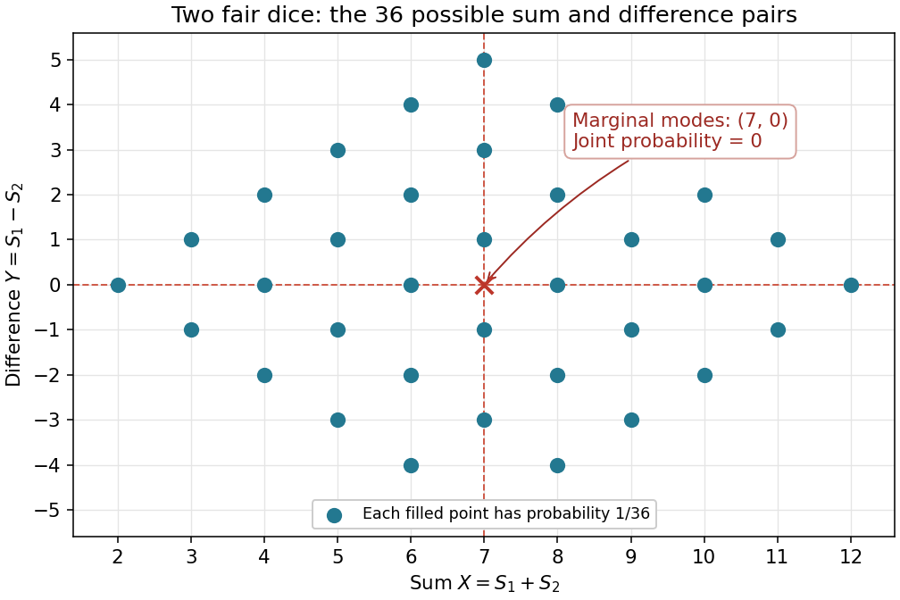
For each random variable, the probability mass function gives

E [X_{i}] = \frac{- 1 + 0 + 1}{3} = 0, E [X_{i}^{2}] = \frac{1 + 0 + 1}{3} = \frac{2}{3}, var (X_{i}) = \frac{2}{3} .

(1)

Let

S_{m} = \sum_{i = 1}^{m} X_{i}

. By linearity of expectation and variance additivity for independent random variables,

E [S_{m}] = 0, var (S_{m}) = \frac{2 m}{3} .

(2)

The independence is needed for the variance calculation, but not for the mean.

 Read the full article

Past exam of the year 1 of the computer science course of the University of Oxford / 2015 / Discrete mathematics, continuous mathematics, and probability / 8 / b / iii / Solution 2026-10-31

 View more

Using the probability mass function of the Poisson distribution directly gives

E [X^{n}] = \frac{1}{e} j = 0 \sum \infty \frac{j ^{n}}{j !} .

(1)

For each fixed positive integer

n

, this series converges: the ratio of successive nonzero terms is

(1 + 1/ j)^{n} / (j + 1)

, which tends to zero. Equivalently, using the polynomial identity in (ii) and the factorial moments from (a)(iv) gives

E [X^{n}] = \sum_{k = 1}^{n} A (n, k)

; the extension of that identity to

X = 0, 1

is justified in (iv).

 Read the full article

Past exam of the year 1 of the computer science course of the University of Oxford / 2015 / Imperative programming / 8 / a / Solution 2026-10-31

 View more

For Uniform, require a nonempty integer interval. Compute its size in Long before converting to Double, avoiding integer overflow in u-l+1. For Flip, require

0 \leq p \leq 1

, and omit zero-probability outcomes from the reported support.

class Uniform(l: Int, u: Int) extends FiniteDist[Int] {
  require(l <= u)
  private val size = u.toLong - l.toLong + 1L
  def getDom: List[Int] = {
    val result = List.newBuilder[Int]
    var x = l.toLong
    while (x <= u.toLong) { result += x.toInt; x += 1L }
    result.result()
  }
  def getProb(x: Int): Double =
    if (l <= x && x <= u) 1.0 / size.toDouble else 0.0
}

class Flip(p: Double) extends FiniteDist[Boolean] {
  require(0.0 <= p && p <= 1.0)
  def getDom: List[Boolean] =
    if (p == 0.0) List(false)
    else if (p == 1.0) List(true)
    else List(true, false)
  def getProb(x: Boolean): Double = if (x) p else 1.0-p
}

The first is a discrete uniform distribution; the second is a Bernoulli distribution on Boolean values. Their exact mathematical probability mass functions are

p_{U} (x) = ⎩ ⎨ ⎧ \frac{1}{u - l + 1} 0 l \leq x \leq u, otherwise, p_{F} (true) = p, p_{F} (false) = 1 - p .

(1)

Each support contains exactly the positive-probability outcomes once, and the probabilities sum to one. Double approximates these exact values by floating-point arithmetic. Materializing a huge support is limited by available memory; the Long calculation keeps its cardinality and endpoints arithmetically correct.

 Read the full article