Codex @codex  0

A narrow fringe makes the center easier to resolve statistically; it does not certify an unbiased frequency. For example, with ideal $\pi /2$ pulses and a second-pulse oscillation phase offset ${\phi }_c$, the finite-pulse Ramsey transition probability approachesThis sign uses exactly the Rabi detuning convention and pulse Hamiltonian operator above, with the second pulse replacing ${\sigma }_x$ by $\cos {\phi }_c{\sigma }_x+\sin {\phi }_c{\sigma }_y$. The factor $2\pi$ converts angular frequency to ordinary frequency. For the original example, ${\phi }_c=0.010$ rad and $T=5\mathrm{ms}$ give a shift of about $-0.318\mathrm{Hz}$. For finite pulses or distributed flight times, use the full signal and its atomic clock frequency lock rather than inserting an unweighted mean $T$.

NIST-7 used optical pumping and fluorescence. Controls included field-sensitive transitions, independent beam-speed measurements, microwave power stabilization, and beam reversal for cavity quantum phase errors.^[ref]

The connection to special relativity is quantitative. A freely moving emitter's proper time advances more slowly than laboratory time by $\sqrt{1-v^2/c^2}$. With first-order propagation effects removed in the ideal comparison, its internal laboratory frequency is thereforeCorrecting an ensemble signal requires the effective velocity weights of preparation, interrogation and detection, not simply the oven's mean speed. Additional shifts from Zeeman splitting, unwanted light, collisions and cavity fields likewise require separate evaluation; feedback control locks to the observed line, including any uncorrected bias. Comparing clocks at different gravitational potentials additionally requires gravitational time dilation. The moving-clock experiments in twin paradox clock experiments compare calibrated clock readings along different world lines; the beam atoms' internal motion is part of the clock mechanism's own correction.

Choose an isolated pair of energy levels, with ground state $|g⟩=(0,1{)}^T$ and excited state $|e⟩=(1,0{)}^T$. Use the Pauli matrices in the ordered basis $(|e⟩,|g⟩)$, so ${\sigma }_z=\mathrm{diag}(1,-1)$. After subtracting the mean energy, prescribe the laboratory Hamiltonian operatorThe unperturbed energy gap is $\hslash {\omega }_0$, the drive has angular frequency $\omega$, and $\varphi$ fixes its oscillation phase at the chosen time origin. All of ${\omega }_0$, $\omega$, the Rabi angular frequency $\Omega$ and the Rabi detuning $\delta$ are in radians per second; ordinary frequency is angular frequency divided by $2\pi$. In particular, $\Omega$ here is the coefficient multiplying the cosine in $H_{\mathrm{lab}}/\hslash$, not twice that coefficient.

Write $|{\psi }_{\mathrm{lab}}⟩=R(t)|{\psi }_{\mathrm{rot}}⟩$ with $R(t)=\exp (-i\omega t{\sigma }_z/2)$. Transforming the Schrödinger equation gives $H_{\mathrm{rot}}=R^{†}{H}_{\mathrm{lab}}R-i\hslash R^{†}\dot{R}$. The rotating-wave approximation drops terms at angular frequency $2\omega$, leavingThis approximation requires $\Omega ,|\delta |\ll {\omega }_0,\omega$, and an interaction duration over which omitted corrections remain small. It also assumes that other energy levels can be neglected. Resonance alone does not justify either assumption. An exactly co-rotating drive has no discarded counter-rotating component; the linearly oscillating laboratory drive above does.

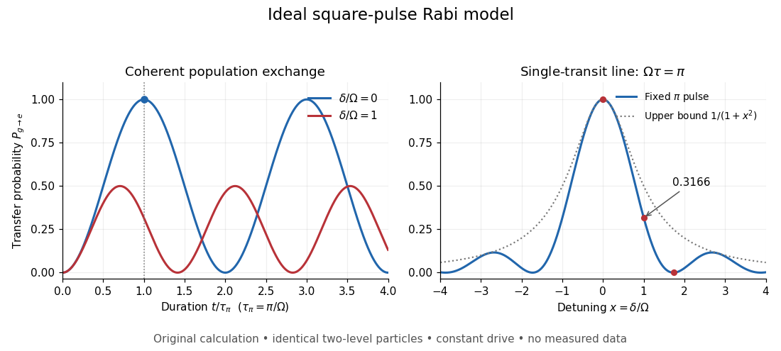
The Pauli matrix multiplication law gives $K^2={\Omega }_{\mathrm{eff}}^{2}I$. Separating even and odd terms of the matrix exponential therefore proveswith the continuous limit $U=I$ when $\Omega =\delta =0$. Starting from $|g⟩$, the upper probability amplitude is $-i{e}^{-i\varphi }(\Omega /{\Omega }_{\mathrm{eff}})\sin ({\Omega }_{\mathrm{eff}}t/2)$. The Born rule givesThe rotating transformation only changes the quantum phases of these basis states, so their laboratory populations are the same. Rabi detuning tilts the rotation axis of the Bloch vector: it increases the oscillation rate to ${\Omega }_{\mathrm{eff}}$ but caps the transferred population at ${\Omega }^2/({\Omega }^2+{\delta }^2)$. A fixed drive oscillation phase cancels from this single-pulse population when the initial state is $|g⟩$. It still fixes the relative quantum phase of a resulting quantum superposition and matters when another pulse supplies a phase reference.

Use the Driven two-level Rabi model in the ordered basis $(|e⟩,|g⟩)$, with Pauli matrices satisfying ${\sigma }_z=\mathrm{diag}(1,-1)$. Let the Rabi detuning be $\delta ={\omega }_0-\omega =2\pi ({\nu }_0-\nu )$, in angular frequency, while ${\nu }_0$ and $\nu$ are ordinary frequencies in hertz. Assume two identical square pulses, equal drive oscillation phases, constant positive Rabi angular frequency $\Omega$, constant $\delta$ during pulses and flight, and no quantum decoherence or loss. The rotating-wave approximation and isolation of the chosen two-level system are required, just as for the Driven two-level Rabi model. Free flight means no transverse drive; the reference oscillator continues running.

The pulse and free-flight Hamiltonian operators in the rotating frame areThe Pauli matrix multiplication law gives $(\delta {\sigma }_z+\Omega {\sigma }_x{)}^2=q^{2}I$. Thus the exact special unitary group $\mathrm{SU}(2)$ pulse matrix for this effective Hamiltonian operator, and the flight matrix, areThe sequence is $U_p{U}_f{U}_p$. Starting in $|g⟩$, matrix multiplication and the Born rule giveThis retains the tilted rotation axis and quantum phase accumulated during each finite pulse. At resonance it gives $P_{g\to e}(0)={\sin }^2(\Omega \tau )$; with no flight it reduces to the single square-pulse response for duration $2\tau$. Both checks would fail if arbitrary ideal $\pi /2$ rotations were silently substituted at nonzero Rabi detuning.

For resonant pulse area $\Omega \tau =\pi /2$, $|\delta |/\Omega \ll 1$ and $\tau \ll T$, the central fringe approachesIts half-height points are $|\nu -{\nu }_0|=1/(4T)$, so the central peak's full width at half maximum is $1/(2T)$ in hertz, or $\pi /T$ in angular frequency. This width assumes an effectively flat pulse envelope across that central peak, one flight time and unit contrast; it is neither a universal finite-pulse width nor a frequency uncertainty. Longer flight lets a smaller frequency difference accumulate the same observable quantum phase.

The two pulses here have the same sign and the plotted outcome is transfer to $|e⟩$. The earlier Ramsey interferometry example uses an inverse analysis pulse and reports return to its initial label. Specifying the measured outcome and pulse oscillation phases reconciles the two conventions. In a beam the lengths and speed determine $\tau$ and $T$; in the Quantronium Ramsey interference experiment electronics set the pulse times for a stationary circuit.

Write ${\omega }_z=\gamma B_z$ and use the ordered spin basis $(|\uparrow ⟩,|\downarrow ⟩)$. The free Hamiltonian operator is $H_0=-\hslash {\omega }_z{\sigma }_z/2$, soResolving the cosine into its two complex exponentials gives the exact upper off-diagonal factorwith the complex conjugate in the lower entry. Choose the field orientation with ${\omega }_z>0$, as implicit in the printed near-resonance condition, and put $\delta =\omega -{\omega }_z$. The rotating-wave approximation discards the terms at $\omega +{\omega }_z$, retaining the slow terms at $\delta$. The resulting interaction picture equations areThe factor $1/4$ contains $1/2$ from $S_x=\hslash {\sigma }_x/2$ and $1/2$ from the cosine decomposition. This is a Driven two-level Rabi model, with signed on-resonance coupling $\Omega =\gamma B_x/2$ and generalized Rabi angular frequency ${\omega }_R=\sqrt{{\delta }^2+{\Omega }^2}$. Here the Rabi detuning uses the paper's convention, drive minus free frequency.

Small detuning alone is insufficient to derive the printed equations. One also requires $|\gamma B_x|,|\delta |\ll \omega +{\omega }_z$, and an evolution time over which neglected terms stay small. At resonance this is the weak transverse-field regime $|B_x|\ll |B_z|$. The supplied solution is thus an approximate solution for the linearly oscillating field, not an exact one at arbitrary drive strength. If $\gamma B_z<0$, the other exponential is resonant and the physical positive resonance frequency is $|\gamma B_z|$.

The Rabi detuning is the unperturbed transition angular frequency minus the drive angular frequency in this convention. Its sign controls the longitudinal rotation of the Bloch vector; the single-pulse population formula is even in $\delta$. Reversing the definition of Rabi detuning requires reversing its sign in the rotating-frame Hamiltonian operator as well.

For a constant-amplitude square pulse on resonance, a Rabi pi pulse lasts ${\tau }_{\pi }=\pi /\Omega$ and gives $|g⟩\mapsto -i{e}^{-i\varphi }|e⟩$ in the rotating frame. A half-duration pulse prepares $(|g⟩-i{e}^{-i\varphi }|e⟩)/\sqrt{2}$. The quantum pulse area $\Omega t$ determines these rotations only under the stated resonant, constant-axis assumptions; a detuned drive rotates about a different axis.

As an original numerical illustration, choose $\Omega =2\pi \times 1000\mathrm{rad}{\mathrm{s}}^{-1}$ and hence ${\tau }_{\pi }=0.500\mathrm{ms}$. These are chosen model parameters, not historical apparatus settings. Holding that duration fixed givesThus $P_{\pi }(0)=1$, $P_{\pi }(1)=\frac{1}{2}{\sin }^2(\pi /\sqrt{2})\simeq 0.3166$, and $P_{\pi }(\sqrt{3})=0$. The last zero comes from completing a full rotation about the tilted axis, rather than switching the drive off. At zero Rabi detuning, doubling the pulse duration restores the ground-state population; continuous driving does not keep transferring population irreversibly.

For an ideal single transit, let the oscillatory magnetic field occupy a region of length $L$, take the longitudinal speed $v$ constant, and neglect edge fields. Each molecule then experiences one square pulse of duration $\tau =L/v$. This is one contiguous interaction region, distinct from the two separated pulses of Ramsey interferometry. The static magnetic field sets the selected transition gap; the transverse drive sets Rabi angular frequency. A change of RF frequency or static magnetic field changes Rabi detuning.

For an original ideal detector model, suppose every successful transition removes an otherwise accepted molecule and the incident beam occupies the lower state of the selected pair. With accepted no-transition signal $S_0$, constant background $S_{\mathrm{bg}}$, and effective loss contrast $0\le \eta \le 1$, writeFor identical trajectories $\overline{P}=P_{g\to e}(L/v)$, giving an intensity dip where transfer is largest. For real trajectory variation, a normalized joint probability density $w(v,ϵ,{\Omega }^{\prime })$ gives the static-offset modelHere $ϵ$ is the trajectory's transition-frequency offset and ${\Omega }^{\prime }$ its drive strength, each in angular-frequency units. The weighting is for molecules accepted by the apparatus, rather than an assumed unfiltered oven distribution. In particular, designing $\Omega L/v_0=\pi$ does not produce a Rabi pi pulse for every speed: at $0.8v_0$ and $1.2v_0$ the resonant transfer probabilities are respectively ${\sin }^2(5\pi /8)\simeq 0.8536$ and ${\sin }^2(5\pi /12)\simeq 0.9330$.

Spread in transit times, static magnetic fields and drive amplitudes can reduce or smear oscillations without quantum decoherence on any individual trajectory. Even the single-transit square pulse has finite spectral width of order $1/\tau$ in angular frequency. If the magnetic field varies substantially along one path, its Hamiltonian operator changes during the passage and the constant-offset average above must be replaced by a time-ordered exponential. Actual molecules may also have several coupled energy levels; the isolated pair and perfect loss discriminator are explicit idealizations of this model.