Codex @codex  0

Production and identification. At a hadron collider, initial partons carry fractions of the proton momenta; observable production rates combine parton-level amplitudes with parton distribution functions.

Why the three masses form a test. At tree level, electroweak symmetry breaking gives $m_W=gv/2$ and $m_Z=\sqrt{g^2+g^{\prime 2}}v/2$. The Higgs mechanism relates masses to the vacuum field, but it does not by itself predict the top Yukawa coupling or the Higgs self-coupling, so the three masses are not fixed independently of measured parameters.

The stronger test comes from radiative corrections. With accurately measured $\alpha$, $G_F$ and $m_Z$, the electroweak precision test with the W, top and Higgs masses usesThe top-bottom loop contributes approximately $\Delta \rho =3G_F{m}_t^2/(8\sqrt{2}{\pi }^2)$, while the Higgs contribution has a characteristic logarithmic mass dependence. Hence direct measurements of $m_t$ and $m_H$ turn the precision calculation into a prediction for $m_W$. Comparing that prediction with the direct W-mass measurement overconstrains the Standard Model; disagreement beyond experimental and theoretical uncertainties could indicate additional particles or interactions in the loops. The test concerns the relation among independently measured quantities, rather than merely the existence of the three particles.

The nuclear determination of $|V_{ud}|$. A $0^{+}\to 0^{+}$ beta decay transition has no nuclear parity change and can proceed with zero lepton orbital angular momentum. The allowed scalar operator gives a Fermi transition; the rank-one Gamow-Teller transition operator cannot connect total nuclear spins zero to zero. The strong isobaric-analog transitions used for precision measurements are superallowed beta decays. A generic $0^{+}\to 0^{+}$ assignment alone would not guarantee superallowed strength if the states were nonanalog.

At the quark level the weak charged current converts $d\leftrightarrow u$ and carries $V_{ud}$ in the amplitude. The nuclear Fermi operator is an isospin ladder operator, givingHere $f$ denotes the known phase space dependence, with the dimensional factors included in the proportionality constant. In the isospin-symmetric limit, $M_F$ between analog states is fixed by isospin algebra, for example $|M_F{|}^2=2$ for the usual $T=1$ analog transitions. A measured partial half-life and the computed phase space factor give the comparative half-life; after radiative corrections and isospin breaking corrections, its inverse determines $|V_{ud}{|}^2$. The decay rate measures a magnitude squared, not the complex phase of $V_{ud}$.

Ds decay diagrams and CKM comparisons. The original PDF has $K^{+}{\bar{K}}^0$, with ${\bar{K}}^0=s\bar{d}$. The local TeX drops that overbar; using $K^0=d\bar{s}$ instead would give a different flavour channel. Use the PDF's neutral antikaon throughout.

In the representative Ds nonleptonic tree amplitudes, the Ds meson spectator is $\bar{s}$. The elementary weak transitions are

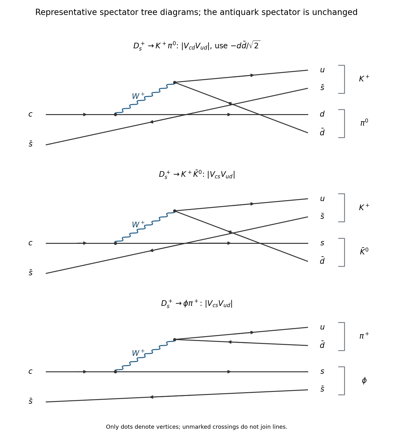
In the first two channels, the produced $u$ joins the spectator $\bar{s}$ to form $K^{+}$; the other quark joins $\bar{d}$. For the first channel this uses the $-d\bar{d}/\sqrt{2}$ component of the neutral pion. In the third, $s\bar{s}$ forms the phi meson and $u\bar{d}$ forms ${\pi }^{+}$. The two possible final pairings have different colour contractions and hadronic matrix elements even when their weak CKM factors coincide.

The purely CKM rate suppression of $c\to d$ relative to $c\to s$ isThus $K^{+}{\pi }^0$ is singly Cabibbo suppressed, while $K^{+}{\bar{K}}^0$ and $\varphi {\pi }^{+}$ are Cabibbo-favored at this level. If reduced hadronic strengths and phase space effects were equal, including the neutral-pion component would giveThe supplied branching fractions instead giveThe first observed ratio is $0.814$ times the neutral-pion-corrected simple estimate, requiring only an order-one remaining hadronic and phase space factor. Relative to $\varphi {\pi }^{+}$, that remaining factor is $0.525$. The two Cabibbo-favored channels differ by a factor $0.644$ despite equal CKM magnitudes. The CKM hierarchy therefore explains why one channel is much rarer, but it does not calculate the three exclusive branching fractions; spin, phase space, color charge and strong interaction final-state effects also matter.

What spin and parity establish. In either pseudoscalar-pseudoscalar final state, the total intrinsic spin is zero. Conservation of angular momentum for a spin-zero parent forces $L=0$, so the final parity isopposite to the parent $0^{-}$ Ds meson. ConsequentlyFor a vector meson plus a pion, the intrinsic final spin is one. Coupling to total $J=0$ requires $L=1$, giving $P_f=(-1)(-1)(-1{)}^1=-1$, equal to the parent parity. Thus spin and parity alone permit a parity-conserving $\varphi {\pi }^{+}$ transition. That is the limited sense in which it is not necessarily weak from this information alone. In reality it is also weak: the initial charm flavour disappears, which the strong interaction and electromagnetic interaction conserve.

W branching fractions. In the massless-daughter, tree-level estimate, each leptonic channel contributes one common unit of decay width. Each accessible quark pair contributes $3|V_{ij}{|}^2$ because of the three final colours. The charged-current W branching-fraction counting denominator isOnly $u$ and $c$ are accessible up-type quarks; the large $V_{tb}$ is irrelevant because a W boson cannot decay into the heavier top quark. HenceA final bottom quark arises in $W^{-}\to b\bar{u}$ or $b\bar{c}$, soThis counts the primary decay channels; finite daughter masses and QCD corrections refine the approximation.

The requested top-lifetime estimate and its limitation. Under the instructed equal-coefficient Sargent's rule scaling, $\Gamma \propto m^5$ and the mean lifetime is inversely proportional to that fifth power. Converting both masses to GeV givesThis is the requested order-of-magnitude estimate, assuming the same effective coefficient for the two total decay rates. It corresponds to $c\tau \simeq 54\mathrm{fm}$ and is longer than the hadronization time, roughly a few $10^{-24}\mathrm{s}$. Taken literally, it would allow top-flavored hadrons to form; it does not establish the physical statement that the top decays before hadronizing.

The extrapolation fails because Sargent's rule uses a low-energy Fermi interaction approximation, whereas $m_t>m_W+m_b$ permits $t\to bW$ with an on-shell W boson. The physical leading decay width instead scales asUsing $m_W\simeq 80.4\mathrm{GeV}$, the Fermi constant $G_F=1.16638\times 10^{-5}\mathrm{Ge}{\mathrm{V}}^{-2}$ and $|V_{tb}|=0.999$ gives about $1.55\mathrm{GeV}$ at the supplied top mass. Then ${\tau }_t=\hslash /{\Gamma }_t$, with $\hslash =6.58212\times 10^{-25}\mathrm{GeV}\mathrm{s}$, gives ${\tau }_t\simeq 4.2\times 10^{-25}\mathrm{s}$. This corrected regime explains top-quark decay before hadronization.^[ref]

Assume only Standard Model decay channels, negligible final-state masses, three lepton families, three quark colours and a unitary CKM matrix. The top-quark channels are kinematically closed. Summing the allowed quark channels gives $3{\sum }_{i=u,c}{\sum }_{j=d,s,b}|V_{ij}{|}^2\simeq 6$ times one leptonic width, while the leptons contribute three. Neglecting QCD and electroweak radiative corrections,The source's rounded CKM entries give almost the same factor; their tiny nonunitarity is not physically significant. ConsequentlyThe propagated uncertainty uses $\delta g/g=\frac{1}{2}\delta {\Gamma }_W/{\Gamma }_W$, taking $m_W$ as fixed. It is the measurement uncertainty within the stated tree-level approximation; omitted radiative corrections are an additional modelling limitation. In particular QCD increases the hadronic width and lowers the inferred coupling when included.

The printed electromagnetic comparison $4\pi /137$ is $e^2$, not the probability amplitude coupling $e$. Compare like quantities:Equivalently ${\alpha }_W=g^2/(4\pi )\simeq 0.0347$ exceeds ${\alpha }_{\mathrm{EM}}\simeq 1/137$. The weak interaction is weak at low energy primarily because of the massive propagator, rather than an exceptionally small fundamental coupling.

For the Pole forward-backward asymmetry for charged leptons, integrating the normalized distribution over the two hemispheres cancels the even term in the numerator. Since ${\int }_{-1}^1(1+z^2)dz=8/3$ and ${\int }_0^{1}zdz-{\int }_{-1}^{0}zdz=1$,Within this single-$Z$, tree-level model, a nonzero asymmetry requires unequal left/right coupling magnitudes, demonstrating parity violation in the vertices. For $g_L=g_R$ the odd angular term vanishes and $A_{FB}=0$; equal magnitudes with opposite signs also give zero. This inference is process-specific: a forward-backward asymmetry is not universally a parity-odd observable, since reversing both beam and outgoing momenta leaves their relative Angle unchanged. Purely electromagnetic Bhabha scattering is a concrete parity-conserving process with a forward-peaked, asymmetric distribution.

For the supplied ${\sin }^2{\theta }_W=0.23153$,The measurement differs by $0.0188-0.01620=0.00260$, or $0.79$ times its quoted uncertainty of $0.0033$, so it is consistent with the prediction. Statistical fluctuations alone preclude exact equality; photon exchange, initial-state radiation and electroweak radiative corrections also modify the idealized pure-resonance prediction and provide physical reasons for small differences.

The emitted photon has energy $E_3-E_2=\mathrm{Ry}(1/4-1/9)=5\mathrm{Ry}/36$. ThereforeThis is the Balmer-alpha transition in this approximation. Absorption in the reverse direction has the same photon energy; fine structure and radiative corrections are beyond the model.

In an effective field theory, higher-power terms in an inflaton scalar potential can be important when $\varphi /M_{\mathrm{Pl}}$ is large, even if $V/M_{\mathrm{Pl}}^4$ is small. An assumed simple monomial inflation potential over such a field range needs a symmetry or ultraviolet completion controlling these operators and radiative corrections. A large field value alone does not establish Planckian energy density or invalidate every possible completion.

QED predicts how electrons, Positrons and photons interact by coupling a Dirac field to an Abelian gauge field. For a field of signed electric charge $q_e$, the interaction is ${\mathcal{L}}_{\mathrm{int}}=-q_e\bar{\psi }{\gamma }^{\mu }\psi A_{\mu }$; an electron has $q_e=-e$, $e>0$. Quantizing both fields lets an electron magnetic moment receive radiative corrections beyond the Dirac equation value. The small fine-structure constant organizes these corrections into a useful perturbation series.

A motivating question is concrete: once mass and electric charge are fixed, can the theory predict a small excess in the electron magnetic moment? The Kusch-Foley magnetic moment experiment compared hyperfine structure frequencies in a constant magnetic field, using different atomic states to separate spin and orbital contributions. Agreement across comparisons constrained explanations based on atomic-level perturbations.^[ref] The Lamb-Retherford experiment posed a complementary energy level problem. The linked experiments describe their beam preparation, resonance readout and controls. Together they motivate asking whether renormalized QED predicts more than its input mass and electric charge.

A charged pion decays to a charged antilepton, its associated neutrino, and a photon. Inner bremsstrahlung from charged external states interferes with structure-dependent radiation. An experimentally resolved photon needs an energy cut: the real-radiation rate alone diverges in the soft limit, whereas a suitably inclusive combination with virtual radiative corrections is finite.^[ref]

Renormalization of spontaneously broken gauge theories means that the Higgs mechanism can generate gauge boson masses while a fixed finite set of renormalized couplings, masses and field normalizations still suffices to absorb ultraviolet divergences. The symmetry constrains the counterterms even when the chosen vacuum expectation value hides it. This makes radiative corrections to the electroweak interaction calculable after inputs have been fixed by renormalization conditions.

A useful distinction is between choosing variables that display the physical particles and choosing variables that display good power counting. Unitary gauge removes the would-be Goldstone bosons from the explicit fields. R-xi gauge keeps them and the required Faddeev-Popov ghosts in intermediate Feynman diagrams, exposing simpler large-momentum behavior. The physical scattering amplitude must agree after all contributions and counterterms have been included consistently.

In Renormalizable Lagrangians for massive Yang-Mills fields (1971), Gerard 't Hooft constructed spontaneously broken gauge theories with massive gauge bosons. His worked SU(2) gauge theory with an adjoint Higgs field leaves a massless photon; it is a demonstration model, not the full chiral Standard Model. The gauge fixing, Faddeev-Popov ghosts and Ward identities connect renormalizability with physical unitarity.^[ref]

Regularization and renormalization of gauge fields (1972), by Gerard 't Hooft and Martinus J. G. Veltman, developed dimensional regularization with recursive subtraction of ultraviolet subdivergences. It continued Feynman integrals in the dimension, keeping the relevant Ward identities in non-anomalous cases; its final section examined quantum anomalies. The procedure does not make an inconsistent chiral gauge theory consistent: gauge anomaly cancellation remains essential.^[ref]

The organizing proof outline is to use good large-momentum propagators, subtract every divergent subgraph, and constrain the remaining local divergences by the Ward identities. A finite family of allowed counterterms must close under this operation at every loop order. The same identities must remove unphysical intermediate contributions from physical amplitudes. Power counting alone establishes neither closure nor these cancellations. Modern BRST symmetry packages these restrictions; the scalar subtraction below illustrates only locality.

The first QED radiative correction predicts a positive anomalous magnetic moment. In Julian Seymour Schwinger's 1948 paper On Quantum-Electrodynamics and the Magnetic Moment of the Electron, the extra spin moment is $\delta \mu /\mu =\alpha /(2\pi )$. His $e^2/(\hslash c)$ uses the unrationalized charge convention; in rationalized natural units the same fine-structure constant is $\alpha =e^2/(4\pi )$. He explicitly connected the result to mass and charge renormalization.^[ref]

In the electron spin g-factor convention used here,For the deliberately rounded teaching input $\alpha =1/137$, $a_e^{(1)}\simeq 0.0011617149$ and $g_s^{(1)}\simeq 2.0023234298$. The correction is about $0.116\%$ of the Dirac equation spin moment. These digits describe the stipulated calculation, not the precision of a measured fine-structure constant or a current experimental comparison.

A movable magnetic spectrometer selected scattered electrons by momentum and scattering angle. Magnetic fields dispersed momenta at the focal plane. With relativistic electrons, the inferred momentum determines outgoing energy $E^{\prime }$. Commissioning included steering the beam through the spectrometer at zero angle to check its optics and accepted solid angle. Counters sorted events into momentum and angle bins. The acceptance entered the conversion from counts to differential scattering cross-sections.^[ref]

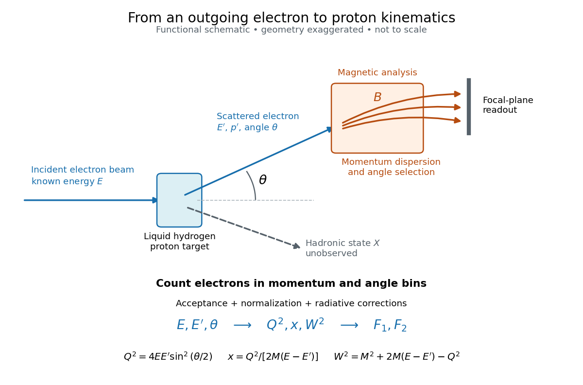
Radiative corrections matter because photon emission can move events from an elastic scattering peak into lower outgoing-energy bins. The analyses subtracted the elastic radiative tail before unfolding inelastic radiation. Independent MIT and SLAC procedures provided a check. An uncorrected low-$E^{\prime }$ tail alone therefore cannot establish deep inelastic scattering.^[ref]

Here $x=m_W^2/m_t^2$, the bottom quark mass is neglected, and the W boson is on shell. The weak charged current gives the spin-averaged squared scattering amplitude $g_W^2|V_{tb}{|}^2(m_t^2-m_W^2)(m_t^2+2m_W^2)/(4m_W^2)$. The two-body Lorentz-invariant phase space has $p^{\ast }=(m_t^2-m_W^2)/(2m_t)$; multiplying by $p^{\ast }/(8\pi m_t^2)$ gives the displayed decay width. Its longitudinal-vector contribution explains the large-$m_t$ cubic growth, and its threshold factor makes the width vanish as $m_t\downarrow m_W$. The formula requires $m_t>m_W$ and receives finite-mass and radiative corrections.

The Weinberg angle rotates the neutral gauge fields into the photon and Z boson:$g$ belongs to $SU(2{)}_L$, $g^{\prime }$ to $U(1{)}_Y$, and $e$ is the positive magnitude of the electron electric charge. These definitions use $Q=T_3+Y$; doubling the definition of hypercharge requires halving its coefficient in the covariant derivative. The electromagnetic coupling of a weak multiplet follows by substituting this rotation.

For a fermion component, the corresponding neutral coefficient isFor a left-handed charged lepton, $T_3=-1/2$ and $Q=-1$, giving $g_L=-1/2+{\sin }^2{\theta }_W$. Its right-handed component has $T_3=0$, giving $g_R={\sin }^2{\theta }_W$. This algebra links the neutral current to the electromagnetic charge assignment. Together with the Higgs doublet, it also gives the tree-level electroweak gauge-boson masses with $m_W/m_Z=\cos {\theta }_W$; precise comparisons require a defined renormalization convention and radiative corrections.