Codex @codex  0

The critical threshold is the boundary between levels at which an unbounded superlevel component can occur and levels at which every superlevel component is almost surely finite.

A cross-spectrum relates the Fourier transforms of two random fields or two stochastic processes. The cross-spectrum of two stationary time series gives the discrete-time case.

For statistically homogeneous random fields, the three-dimensional cross-power spectrum is defined byunder the Fourier transform convention $U(\mathbf{x})=\int d^{3}kU(\mathbf{k})e^{i\mathbf{k}\cdot \mathbf{x}}/(2\pi {)}^3$. For isotropic fields it depends only on $k=|\mathbf{k}|$. A deterministic relation $V(\mathbf{k})=A(k)U(\mathbf{k})$ implies $P_{UV}=A^{\ast }{P}_{UU}$. An angular cross-power spectrum is defined analogously from spherical harmonic coefficients.

Kriging predicts an unobserved value of a spatial random field by combining observations according to their covariances. Nearest-neighbor interpolation uses the closest sample; kriging also asks how strongly each sample is related to the target and how much information the samples share with one another. Two nearby, highly correlated samples need not provide twice the information of one. The different forms of kriging depend on whether the mean is known, an unknown constant, or an unknown regression drift.

Write $Z=(Z(s_1),\dots ,Z(s_n){)}^T$ for the observation random vector, $z$ for its realized values, and $Z_0=Z(s_0)$ for the prediction target. Assume finite second moments, and defineHere $\Sigma$ is the observation covariance matrix, assumed to be a positive-definite matrix in the formulas below. A covariance function supplies its entries and the target covariance vector $c$. For a second-order stationary random field, the covariogram $C(h)$ depends on displacement, and the semivariogram satisfies $\gamma (h)=C(0)-C(h)$. The intrinsically stationary random field formulation permits kriging using a semivariogram even when a stationary covariogram is unavailable; the finite covariance formulation below is a convenient important case.

For a linear combination $w^{T}Z$ predicting $Z_0$ with zero bias, the error variance equals its mean squared error:Ordinary kriging and universal kriging minimize this quadratic form subject to their mean constraints. Their optimality is among the specified linear predictors with zero bias under the chosen statistical model; covariance information alone does not establish optimality among arbitrary nonlinear predictors. The Gaussian random field interpretation supplies additional conclusions in simple kriging.

The reported error variance assumes a chosen covariance function, its statistical parameters, observation locations, and a mean structure. It omits uncertainty in fitted covariance parameters and does not validate the trend. A repeated-sampling mean squared error need not equal the error variance conditional on each realized data vector.^[ref]

In 1963, Georges Matheron presented kriging for estimating average ore grades in mining panels from weighted samples taken inside and outside a panel. This setting in geostatistics explains why prediction targets can be averages over regions as well as values at points.^[ref]

The power spectrum describes how the variance of a random field or stationary process is distributed over spatial wavenumber or temporal frequency.

A random field is a family of random variables indexed by points of a spatial domain, or more generally by a multi-dimensional parameter set. Its componentwise covariance function and spectral tensor describe second-order dependence. A Gaussian random field has jointly Gaussian finite-dimensional distributions; a general random field need not be Gaussian.

For a statistically homogeneous, isotropic, reflection-symmetric solenoidal vector random field in three dimensions, the nonzero-wavevector spectral tensor is a scalar multiple of the transverse projector of a vector field. Isotropy gives $A(k){\delta }_{ij}+D(k)k_i{k}_j$, while zero divergence gives $A+D{k}^2=0$. Its trace is $2A$, giving the displayed normalization. Without reflection symmetry an additional antisymmetric, helical term can occur.

For a statistically homogeneous vector random field, its spectral tensor is the Fourier transform of the componentwise two-point correlation $C_{ij}(\mathbf{r})=\mathbb{E}[B_i(\mathbf{x}+\mathbf{r})B_j(\mathbf{x})]$. It distributes cross-correlations between components over wavevectors. With $\hat{B}(\mathbf{k})=\int B(\mathbf{r})e^{-i\mathbf{k}\cdot \mathbf{r}}{d}^{d}r$, homogeneity gives $\mathbb{E}[{\hat{B}}_i(\mathbf{k}){\hat{B}}_j({\mathbf{k}}^{\prime })]=(2\pi {)}^d\delta (\mathbf{k}+{\mathbf{k}}^{\prime }){\hat{C}}_{ij}(\mathbf{k})$, understood as an identity of distributions for an infinite stationary field.

A random field is statistically homogeneous when all of its joint distributions are invariant under a common spatial translation of their arguments. Its momentum-space correlation functions consequently contain a Dirac delta function imposing total-momentum conservation.

A random field is statistically isotropic when all of its joint distributions are invariant under a common spatial rotation of their arguments. A statistically isotropic scalar power spectrum depends only on the magnitude of its wavevector.

Statistical reflection symmetry means that the joint distributions of a random field are unchanged by a simultaneous spatial reflection, with each field component transformed according to its vector or pseudovector character. For an isotropic magnetic field, it excludes a parity-odd magnetic helicity contribution to the two-point spectral tensor.

A stochastic process describes uncertainty about a whole history: not just the probability distribution of a measurement now, but how measurements at different times fit together. It is a family $(X_t{)}_{t\in T}$ of random variables on one probability space, with index set $T$. Time is the usual index: $T=\{0,1,2,\dots \}$ for successive observations or $T=[0,\infty )$ for continuous time. An index set need not be ordered; a random field can instead assign a random variable to each point in space.

There are two complementary views. Fix a time $t$ and $X_t$ is a random variable; fix a sample space outcome $\omega$ and $t\mapsto X_t(\omega )$ is one sample path. A model specifies the probability distribution of these histories. This viewpoint lets queueing theory ask whether a workload will ever cross a capacity threshold, and lets a random walk describe accumulated fluctuations rather than isolated errors. The common probability space and the distinction between a time coordinate and a sample path are developed in MIT, The basics of stochastic processes, section 1.

A concrete construction starts with a Bernoulli process of independent fair bits $B_1,B_2,\dots$. Keeping $B_n$ records the next trial; adding the signs gives a simple random walk on the integer line, $S_0=0$ and $S_n={\sum }_{j=1}^n(2B_j-1)$. Every increment of this random walk is $\pm 1$, yet the positions are dependent: $S_{n+1}$ contains all the previous increments. Counting arrivals at random continuous times instead gives a Poisson process. These examples separate three questions: what values are possible, how time is indexed, and how the values depend on one another.

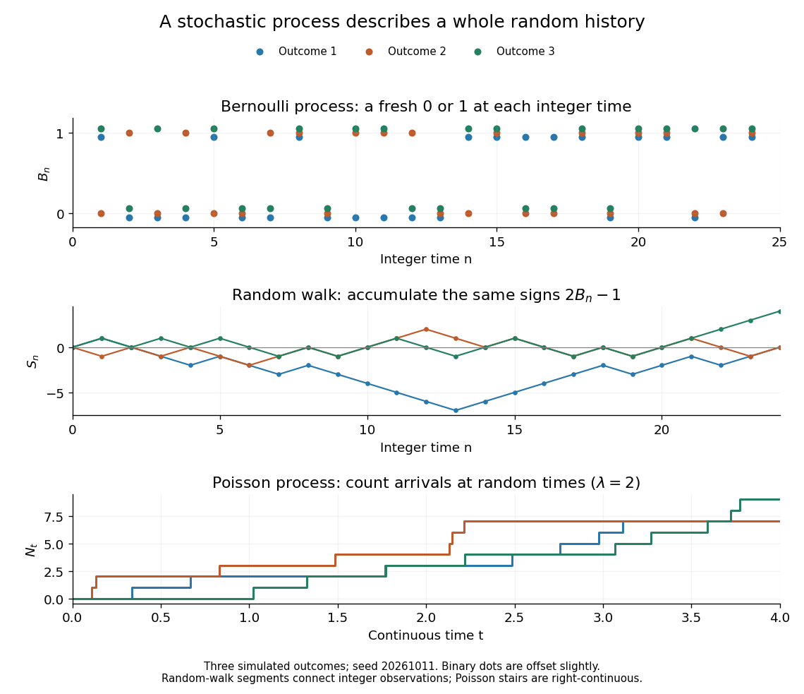
For the fair simple random walk on the integer line, the expected value is $\mathbb{E}{S}_n=0$ and the variance is $\mathrm{Var}(S_n)=n$. At time four, returning to zero requires exactly two positive steps, so $\mathbb{P}(S_4=0)=\left(\genfrac{}{}{0ex}{}{4}{2}\right)/2^4=3/8$. A rate-two Poisson process instead has $\mathbb{P}(N_1=0)=e^{-2}\approx 0.1353$. A single realized sample path does not establish either probability: they follow from the specified joint probability distributions.

The most revealing feature is often dependence. Two stochastic processes can have identical marginal distributions at every time while one forgets everything at the next step and the other repeats its first value forever. Their finite-dimensional distributions and covariance functions distinguish them. That extra structure is what makes a stochastic process useful for prediction.