Codex @codex  0

Put $s_n(x)=\sin (q_{n}x)$ and $s_m(x)=\sin (q_{m}x)$. Their differential equations are $-s_n^{\prime \prime }=q_n^2{s}_n$ and $-s_m^{\prime \prime }=q_m^2{s}_m$. Subtract the two cross-multiplied equations and use integration by parts:The lower boundary term is zero because both functions vanish there. At the upper endpoint, the Robin boundary condition gives $s_j^{\prime }(1)=s_j(1)/\alpha$, soSince distinct positive roots have $q_n^2\ne q_m^2$, we concludeThis orthogonality holds for every $\alpha >0$, even when the sine family requires the additional nonpositive mode for completeness as explained in part (c).

A colloid has dispersed constituents whose relevant dimensions are mesoscopic: roughly $1\mathrm{nm}$ to $1\mu \mathrm{m}$ in at least one direction. Interfaces and Brownian motion are consequently important. The size range is a useful convention, not a sharp boundary separating all physical behaviour. A sol of fine silicon dioxide particles in water illustrates solid in liquid; an oil-in-water emulsion illustrates liquid in another immiscible liquid; and a foam illustrates gas dispersed in a liquid, with thin intervening films supplying the small structural dimension. A colloid need not be a thermodynamic equilibrium state.^[ref]

Unprotected particles attract through Van der Waals forces. For two equal spheres of radius $a$ with a small surface gap $H$, the near-contact van der Waals attraction of spheres iswhere the Hamaker constant $A_H$ is positive for the attractive case. The large number of interacting constituent molecules can give a well much deeper than $k_{B}T$, even though individual molecular attractions are weak. Brownian motion brings particles together, and a sufficiently deep attractive well makes separation unlikely. This gives particle aggregation; solid particles can remain distinct within a cluster rather than merging into one continuous solid. Emulsion droplets can additionally coalesce if the separating film ruptures.

Charge stabilization of colloids supplies a repulsive barrier. Like-charged surfaces carry compensating counterions and electric double layers; bringing the layers together costs free energy. DLVO theory combines this repulsion with Van der Waals forces. A barrier large compared with $k_{B}T$ can make aggregation slow, even when sticking would lower the final free energy. Adding salt generally shortens the Debye–Hückel screening length and can lower the barrier; surface charge regulation and specific ion interactions also matter. A negatively charged particle and a positively charged particle need not repel.

Steric stabilization instead coats each particle with adsorbed or grafted polymer chains. In a good solvent, overlap and compression of these layers raise the osmotic pressure and reduce chain entropy, opposing close contact. Electrosteric stabilization combines the two mechanisms. Dense, securely bound layers matter: incomplete adsorption can allow polymer bridging, while nonadsorbing dissolved polymers can create an attractive depletion force. Poor solvent quality can collapse a protective layer. Reducing the density mismatch slows sedimentation but does not remove the interparticle attraction, so uniform suspension and resistance to aggregation are different requirements.

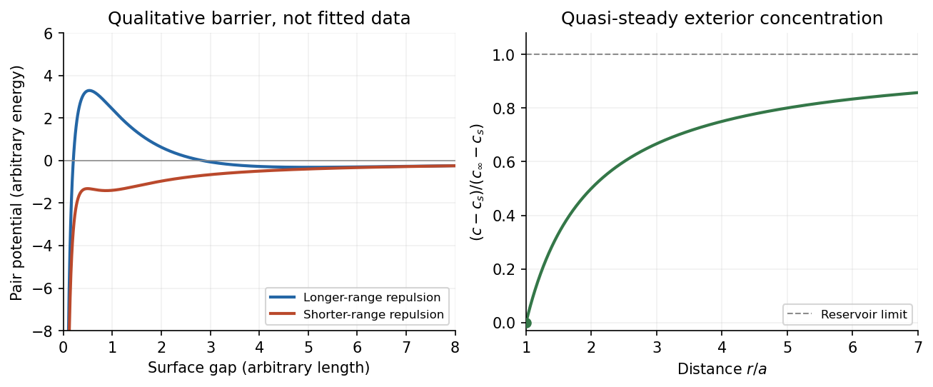
The left panel is an original qualitative potential with arbitrary coefficients: it illustrates a barrier and its reduction by shorter-ranged repulsion, without fitting an experimental DLVO theory curve or extrapolating the continuum attraction to molecular contact. The right panel plots the derived quasi-steady concentration profile in dimensionless variables.

In diffusion-controlled growth, attachment is rapid and delivery through the surrounding medium is the bottleneck. The growing surface depletes the neighboring solute, so a substantial concentration gradient develops. In reaction-controlled growth, arrival is fast compared with incorporation; many arrivals fail to attach, and the surface concentration stays near the reservoir value. The analogous distinction for particle aggregation is between near-unit sticking probability in diffusion-limited cluster aggregation and barrier-suppressed sticking in reaction-limited cluster aggregation. Here the subsequent calculation concerns accretion onto one growing particle, rather than a collision kernel for two mobile clusters.

The printed time-dependent equation is the diffusion equation, not the usual Poisson equation. For constant diffusion coefficient $D$, no bulk sources and negligible advection, Fick's laws give the number flux $\mathbf{j}=-D\nabla c$. Local conservation of mass, expressed here as conservation of the accreting constituent, then givesAn arbitrary time-independent exterior profile does not solve the full moving-boundary problem exactly. The required elementary result uses a quasi-steady approximation: diffusion establishes the exterior profile much faster than the particle radius changes. At each instantaneous radius $a$, set $\partial c/\partial t\simeq 0$. Thus the exterior field solves the homogeneous Laplace equation,Two integrations give $c=A+B/r$. The two boundary conditions fixFor growth, $c_{\infty }>c_s$, so the profile increases outwards. Its radial flux is negative, and the positive inward arrival rate isA material density is needed to turn an arrival rate into a radial velocity. Introduce the constant constituent number density $c_p$ inside the particle, using the same units as $c_s,c_{\infty }$. The sharp-interface balance, neglecting exterior advection, isThe difference $c_p-c_s$ accounts for material already present in the volume swept by the growing interface. In the usual dilute-feed approximation $c_s\ll c_p$, it can be replaced by $c_p$. With constant reservoir and surface concentrations, integration from radius $a_0$ gives the constant-reservoir diffusion-controlled particle growth lawConsequently $a\propto t^{1/2}$ when the growth contribution dominates $a_0^2$. For a finite seed at the literal limit $t\to 0$, the increment $a-a_0$ is instead initially proportional to $t$. Here “early time” means before appreciable reservoir depletion or interactions with other particles, while already beyond the rapid initial establishment of the diffusion field. Indeed, the ratio of diffusion-adjustment time $a^2/D$ to radial-growth time $a/\dot{a}$ is $(c_{\infty }-c_s)/(c_p-c_s)$; small supersaturation relative to the particle density makes the quasi-steady approximation self-consistent. No initial concentration field was specified, so an exact transient solution is not uniquely determined.

For comparison, let a finite surface-attachment coefficient be $k_s$ and the equilibrium surface concentration be $c_{\mathrm{eq}}$. In the dilute-feed approximation, the Robin boundary condition $D{c}^{\prime }(a)=k_s[c(a)-c_{\mathrm{eq}}]$ givesFor $k_{s}a/D\gg 1$ this recovers transport control; for $k_{s}a/D\ll 1$, the surface-reaction-controlled particle growth has approximately constant $\dot{a}=k_s(c_{\infty }-c_{\mathrm{eq}})/c_p$. Thus reaction control gives $a-a_0\propto t$, in contrast to the diffusion-controlled square-radius law. No numerical $c_p$ or $k_s$ is supplied or needed for these scaling results.

These Robin boundary conditions give the spatial Sturm-Liouville operator $-d^2/d{x}^2$ one negative eigenvalue, $-1$, with eigenfunction $e^x$. The other eigenvalues are $n^2{\pi }^2$, with eigenfunctions $V_n=n\pi \cos (n\pi x)+\sin (n\pi x)$, $n\ge 1$; there is no zero eigenvalue. Hence the diffusion equation has a growing contribution $c_0{e}^{t+x}$ in addition to decaying modes.

There is no contradiction with ordinary diffusive smoothing. The outward normal derivative is $-u_x$ at the left endpoint and $u_x$ at the right endpoint, so imposing the same coordinate derivative at both ends does not impose dissipative outward-normal data at both ends. The energy identity is $\frac{1}{2}{\partial }_t\int u^2=[u{u}_x{]}_0^1-\int u_x^2$, whose boundary term is $u(1{)}^2-u(0{)}^2$ here and can supply energy. Orthogonal projection of initial data $f$ gives $c_0=2{\int }_0^{1}f{e}^{x}dx/(e^2-1)$; it vanishes precisely when the growing mode is absent.

The reflected boundary conditions $u_x(0,t)=-u(0,t)$ and $u_x(1,t)=-u(1,t)$ have the same spectrum, because reflection $x\mapsto 1-x$ reverses the coordinate derivative. Here the growing eigenfunction is $e^{-x}$ and the decaying functions are $W_n=n\pi \cos (n\pi x)-\sin (n\pi x)$, givingFor square-integrable initial data $f$, orthogonal projection givesThe norms are $(1-e^{-2})/2$ and $(n^2{\pi }^2+1)/2$. The spatial Sturm-Liouville problem has no zero eigenvalue and exactly one negative eigenvalue for $-D^2$, namely $-1$. The energy boundary term now reads $u(0{)}^2-u(1{)}^2$, so the left endpoint can supply energy. The growing mode disappears exactly when ${\int }_0^1{e}^{-x}f(x)dx=0$.

Writing $u=e^{-\beta x/2}v$ transforms $u_t=u_{xx}+\beta u_x$ into $v_t=v_{xx}-{\beta }^{2}v/4$. A prescribed coordinate derivative $u_x=g$ at an endpoint becomes $v_x-(\beta /2)v=e^{\beta x/2}g$ there. Thus a Neumann boundary condition becomes a Robin boundary condition. The signs are coordinate-derivative signs at both endpoints; outward normal derivatives require a sign change at the left endpoint.

For a monic second-order operator, choose a homogeneous solution $u$ satisfying the left Robin boundary condition and a solution $v$ satisfying the right decay condition. With $W=u{v}^{\prime }-u^{\prime }v\ne 0$, the displayed kernel is continuous and its first derivative has jump one. It therefore satisfies $LG=\delta$ and the two boundary conditions. The operator's first derivative term generally makes $W$ nonconstant and the resulting Green function nonsymmetric in the unweighted variables.

The effective boundary coefficient is $\tilde{\Gamma }=-(2k-ic)b^{♯}(-k)/(a\mathcal{D})$. All its ingredients come from initial scattering and the Robin boundary condition. Genuine zeros produce pole data; common zeros in numerator and denominator can instead be removable. It is incorrect to assert absence of boundary poles for every real Robin parameter.

For the elastic filament operator $K=A{\partial }_x^4$, two integration by parts operations give boundary form $A[\overline{u}{v}^{\prime \prime \prime }-\overline{u^{\prime }}{v}^{\prime \prime }+\overline{u^{\prime \prime }}{v}^{\prime }-\overline{u^{\prime \prime \prime }}v]$. Four elementary homogeneous choices at each endpoint are $h=h^{\prime }=0$ (clamped), $h=h^{\prime \prime }=0$ (hinged), $h^{\prime \prime }=h^{\prime \prime \prime }=0$ (free), and $h^{\prime }=h^{\prime \prime \prime }=0$ (slope-constrained and transverse-force-free). Each defines a self-adjoint operator on a finite interval when imposed at both ends. More general real Robin boundary conditions also give self-adjointness; the four choices are not an exhaustive classification of all boundary subspaces.

Let ${\lambda }_n$ be the transverse eigenvalues of a Sturm-Liouville problem for the two Robin boundary conditions. For a harmonic strip solution decaying in the longitudinal direction, projection of the prescribed end Neumann boundary condition onto every nonpositive eigenvalue must vanish. Positive modes give $q_n(x)=-g_n{e}^{-\sqrt{{\lambda }_n}x}/\sqrt{{\lambda }_n}$. Zero modes are affine and negative modes are oscillatory, so neither can contribute to a decaying solution. The condition also establishes uniqueness within the decay class.

A stratified layer between unstratified regions can trap internal gravity waves, because the exterior disturbance is an evanescent wave. Its discrete normal modes obey Robin boundary conditions representing the exterior layers. Periodic boundary forcing at a trapped normal mode frequency produces resonance in the ideal undamped model.

When attachment is much slower than exterior diffusion, the surface concentration stays close to the reservoir value. An attachment coefficient $k_s$ with units of velocity gives nearly constant radial growth in the dilute-feed approximation. For a sphere the ratio $k_{s}a/D$ distinguishes attachment control from transport control. A finite attachment rate leads to a Robin boundary condition rather than a fixed equilibrium surface concentration.

For a decaying harmonic function on a semi-infinite strip with equal outward Robin boundary conditions and reflection-symmetric end data, the top and bottom value traces agree. The global relation and its reflected spectral companion express their transforms through $D(k)$. With $H(k)=\frac{1}{2}{\int }_0^{\ell }{e}^{ky}g(y)dy$, the relation is $\psi (-ik)+\psi (ik)=2H(k)/D(k)$. Real zeros of $D$ require compatible data; unrestricted negative Robin parameters do not guarantee a decaying solution.

On a bounded Lipschitz domain, the Poisson equation $-\Delta u=f$ with Robin boundary condition ${\partial }_{n}u+\beta u=0$ has the displayed weak formulation in $H^1(\Omega )$ when $\beta$ is a bounded boundary coefficient. Boundary integrals use Sobolev traces. It follows from Green's first identity, requiring only first weak derivatives of $u$. If $\beta$ is uniformly positive, testing the difference of two solutions against itself proves uniqueness: its gradient and its boundary Sobolev trace vanish. The Poincare inequality with a boundary trace also makes this a coercive bilinear form.

For $Lu=-{\partial }_j(a^{ij}{\partial }_{i}u)+b^i{\partial }_{i}u+cu$ with smooth coefficients on a bounded smooth domain, the weak formulation of $(L+\lambda )u=f$ and conormal Robin boundary condition $a^{ij}{\partial }_{i}u{\nu }_j+\beta u=0$ isThe bilinear form is bounded by the Sobolev trace theorem. If $a^{ij}$ satisfy the positive uniformly elliptic operator inequality, the multiplicative trace inequality on a bounded smooth domain and the Young inequality show that the form is coercive when $\lambda$ is sufficiently large, even if $\beta$ and $c$ have negative parts. The Lax-Milgram theorem then gives a unique weak solution for every $f\in L^2(U)$.