Gaussian elimination applies elementary row operations to reduce a linear system to triangular form. Dense elimination uses arithmetic operations.
Gaussian elimination solves a linear system by removing one unknown from later equations at each step. Write the coefficients and right-hand side together as an augmented matrix . Apply the same elementary row operations to both parts until the coefficients form a row echelon form; for a square invertible matrix, this gives an upper triangular matrix system. Then back substitution recovers the unknowns from the last equation upward. The useful simplification is that each successive equation involves fewer unknowns, while the set of solutions stays the same.
Why do elementary row operations preserve solutions? Interchanging equations changes only their order. Multiplying an equation by a nonzero scalar can be undone by division. Replacing equation by itself plus times equation , with , can be undone by adding times the unchanged equation . Equivalently, an elementary matrix is an invertible matrix, so if and only if . Applying an operation to without also applying it to loses this equivalence.
At step , choose a nonzero pivot element after any row interchange. For every , form the elimination multiplier and perform the elementary row operation . Its coefficient in column becomes in exact arithmetic. Later operations combine rows that already have zeros in earlier columns, so those zeros survive. If an active column has no nonzero candidate, general row echelon form reduction skips it; a square invertible matrix always has a candidate at each step with suitable row interchanges. Partial pivoting also considers roundoff error when selecting the candidate.[ref]
2.6 Row pivoting. Fundamentals of Numerical Computation by Tobin A. Driscoll and others; §2.6.1, Definition 2.6.1: select the largest absolute candidate; §2.6.3: permute the right-hand side too
For a dense matrix with one right-hand side, the classical algorithm uses arithmetic operations over the real numbers, counting each addition, subtraction, multiplication and division as one. At step , the coefficient update has entries, each costing one multiplication and one subtraction; the elimination multipliers, right-hand-side updates and back substitution contribute lower-order terms. Searching for partial pivoting adds comparisons, and storing the dense coefficients uses space. These assumptions exclude the different storage and work patterns of sparse Gaussian elimination; the exact loop counts appear in LU factorization and solve costs. Here denotes Big O notation.
Recording the same steps as an LU decomposition makes Reusing LU factors for multiple right-hand sides possible. This is useful whenever the coefficients stay fixed while the forcing vector changes: the expensive elimination is done once. The choice of pivot element matters even when the linear system is well conditioned, as Tiny-pivot roundoff in Gaussian elimination demonstrates.
For a band matrix, elimination without pivoting retains bounded lower and upper bandwidths in its triangular factors. A tridiagonal system therefore needs only linear work and storage, as in the Thomas algorithm. Pivoting can change the precise fill pattern and must be included in the bandwidth and cost analysis when required. The inverse need not be banded, so solving through the factors preserves sparsity that explicit inversion would lose.
A fraction-free elimination algorithm for exact determinants. At each stage it divides a cross-multiplied update by the preceding pivot; the determinantal identities underlying the method make this division exact when its pivot assumptions hold. Pivoting handles zero pivots.
Consider this original linear system and its augmented matrix:The first diagonal entry is zero, so it cannot serve as a pivot element. Interchange and to obtain a pivot element of one:This chooses a convenient nonzero entry for exact arithmetic; partial pivoting would instead interchange and , selecting the largest absolute value, two. For our chosen ordering, the first-column elimination multipliers are and . The elementary row operation givesThe next pivot element is two and the next elimination multiplier is . Applying gives the upper triangular matrix systemEvery operation also changed the right-hand side. Back substitution now givesChecking the original equations, rather than only the reduced ones, verifies the answer by matrix multiplication:Thus a zero first diagonal entry was a row-order obstruction, not a singular matrix. Indeed, the diagonal product of the final upper triangular matrix is ; the single row interchange makes , since the two row additions preserve the determinant.
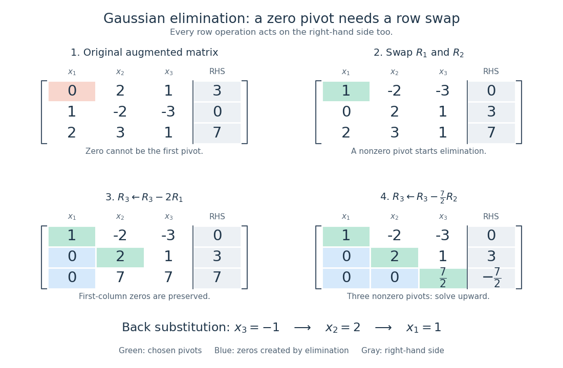
A row interchange supplies the first pivot element; successive elementary row operations create zeros, then back substitution gives
. Details. A pivot element is the current diagonal entry used to eliminate entries below it in Gaussian elimination, after any row interchange. At step it is , where is the current reduced matrix. Computing elimination multipliers requires this entry to be nonzero. A zero pivot element can reflect an unsuitable row order even for an invertible matrix, as Pivoted LU decomposition illustrates.
For , an elimination multiplier is the scalar used in the elementary row operation . This creates a zero below the pivot element. The remaining entries change by for . Storing these elimination multipliers gives the subdiagonal entries of in LU decomposition; later row interchanges must also reorder the already stored coefficients.
Sparse Gaussian elimination solves a linear system by Gaussian elimination while exploiting its sparse matrix structure to avoid storing zeros and performing unnecessary arithmetic operations. The catch is that zeros in the input need not remain zero: eliminating a shared unknown can couple two equations that previously had no direct coupling. These new positions are fill-in, and their number can depend strongly on the order of elimination.
For a real symmetric positive-definite matrix, the usual direct method is a Cholesky decomposition. Choose an ordering, use symbolic factorization to allocate the predicted factor entries, compute their values, then solve two triangular systems. Compressed sparse storage makes the reduced storage useful. General LU decomposition may also need numerical partial pivoting, so an ordering chosen for sparsity can change during factorization.[ref]
Lecture 27: Sparse Gaussian Elimination. Applications of Parallel Computers, CS267, Spring 1996; CS267, Lecture 27, 23 April 1996, Cholesky versus LU Decomposition: distinction between numerical pivot selection and advance ordering, and phases 1–4; Sparse Matrix Storage Schemes
For a fixed ordering, let be the permutation matrix that puts the unknowns in that order. Permute both rows and columns:Here is the lower triangular matrix in the Cholesky decomposition of ; . Forward substitution and back substitution give the original solution. The simultaneous permutation preserves the symmetric positive-definite matrix property because for every nonzero vector . A row permutation alone generally loses the symmetric matrix structure.
The local mechanism is a Schur complement. If the active pivot element is , then for remaining indices ,Even when , two nonzero couplings through make the second term nonzero. Thus the elimination graph removes and joins its remaining neighbors into a clique. The fill-path criterion for symmetric elimination extends this local rule across several steps. The elimination tree organizes the resulting dependencies; the minimum degree algorithm and nested dissection choose orderings to control them.
This connection between graphs and linear systems was already explicit in Donald J. Rose, R. Endre Tarjan and George S. Lueker's 1976 study of fill-in and perfect elimination orderings.[ref]
Algorithmic Aspects of Vertex Elimination on Graphs by Donald J. Rose and others. Abstract: symmetric positive-definite systems, fill calculation for a prescribed ordering, and algorithms for special orderings; publication information, June 1976
Take a star graph with center and four leaves . Let be its Laplacian matrix and the identity matrix. In the order , the original example isFor a nonzero vector , its quadratic form isThus is a symmetric positive-definite matrix and either ordering below admits a Cholesky decomposition. Changing the ordering changes the work, rather than the mathematical solvability.
Center first. Eliminating with pivot element leaves the Schur complementEvery pair of leaves now has coupling : six new edges, hence six undirected fill-in positions. The four remaining vertices form a clique. In the Cholesky decomposition, the first column has and . The rest of the lower triangular matrix is dense. To check that later cancellation does not remove its entries, after leaves have also been eliminated, the active leaf block isIndeed a leaf step sends to . All active off-diagonal entries remain negative. The successive pivot elements in ordinary symmetric Gaussian elimination, equivalently the squared diagonals in the Cholesky decomposition, areThe Cholesky decomposition therefore stores nonzero entries, including its diagonal.
Leaves first. Permute to . Each leaf has only one remaining neighbor, so its elimination changes only the center's diagonal, reducing it by . The successive pivot elements are , and the exact Cholesky decomposition isThere is no fill-in, and only nonzero entries in . This is a concrete instance of leaf elimination of a tree-pattern positive-definite matrix; its general proof explains why the same idea works on every tree pattern. The minimum degree algorithm also chooses a leaf at every nontrivial stage of this particular example, but that success gives no general optimality guarantee.
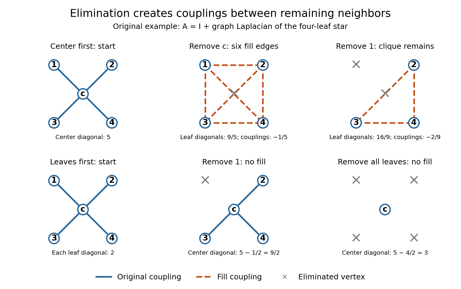
Eliminating the center of a four-leaf star graph creates a clique; eliminating leaves creates no fill-in
. Details. 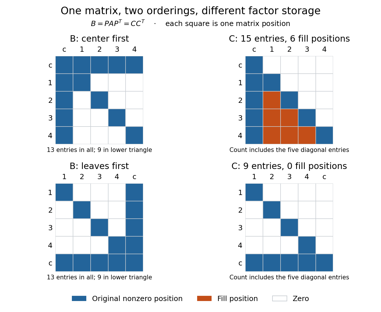
The same symmetric positive-definite matrix has 15 or nine nonzero Cholesky decomposition factor entries, depending on its ordering
. Details. The input has 13 nonzero matrix elements when both symmetric halves are counted, or nine in its lower triangle. The six added undirected edges correspond to six added positions in one triangular factor, or 12 positions if both symmetric halves of the filled pattern are displayed. Comparing all 13 input entries directly with the 15 entries of would mix counting conventions.
Associate an undirected graph with a symmetric matrix's off-diagonal nonzero pattern. Eliminating vertex updates the remaining matrix by . Only pairs of neighbors of can acquire fill-in. If the graph is a tree, remove leaves successively: each eliminated vertex has at most one remaining neighbor, so only a diagonal entry can change. Every Schur complement of a positive-definite matrix is positive definite, so no zero pivot forces a different ordering. Leaf removal therefore constructs a perfect elimination ordering and a fill-free factorization.
Symbolic factorization computes possible nonzero positions and update dependencies from a sparse matrix pattern and ordering before calculating numerical factor values. The elimination graph predicts fill and the elimination tree organizes dependencies. Numerical pivoting or exceptional cancellation can make the computed factor pattern differ from this structural prediction.
For a symmetric factorization in a fixed ordering, the elimination tree assigns the displayed parent to a column of the lower-triangular factor when that set is nonempty. A column with no later entry is a root. The tree records dependencies of descendant updates on later pivots, supports symbolic factor allocation, and exposes parallel subtrees. It describes the factorization ordering, not merely a spanning tree of the original matrix graph.
A vertex separator divides the remaining unknowns into disconnected subdomains. Nested dissection recursively eliminates each subdomain before its separator, keeping interaction localized until late in the factorization. For a regular two-dimensional mesh with unknowns, separators have size ; the resulting direct factorization uses work and storage under the usual geometric separator assumptions.
At each step choose a remaining vertex of minimum degree in the current elimination graph. This heuristic reduces the size of the immediate Schur complement update and often reduces fill-in, but does not guarantee a globally optimal ordering. Its degrees must reflect earlier fill, rather than just the original graph.
Fill-in consists of new nonzero positions created by Gaussian elimination, absent from the original sparse matrix in the same ordering. For a Cholesky decomposition , compare with the lower triangle of , not with the unpermuted input. Each new undirected edge of the elimination graph contributes one structural position in . The sparse elimination of a four-leaf star gives six such positions when the center is eliminated first, and none when the leaves are eliminated first.
Symbolic factorization predicts possible nonzeros from the pattern alone. An initially zero becomes nonzero in a single scalar step if both and are nonzero; however, at later steps several contributions can cancel. For an exact example, letEliminate indices in that order. The first Schur complement, in order , isThe second pivot element updates the entry to . The remaining block is , so all four pivot elements are positive and is a symmetric positive-definite matrix. The elimination graph retains the structural edge , but this exact choice of coefficients makes the numerical entry vanish. A small change to generally removes the cancellation.
Such an exact zero is different from discarding a small value computed with floating-point arithmetic. The symbolic factorization deliberately reserves space for possible entries without depending on special numerical identities. A perfect elimination ordering creates no structural fill-in at all; an ordering with cancellations need not have that property.
For a symmetric sparse matrix, its matrix graph has one vertex per unknown and an edge whenever the off-diagonal entry is structurally nonzero. Simultaneous row and column permutation relabels this graph. Nonsymmetric patterns are instead represented by directed or bipartite graphs when row and column roles must be distinguished.
One step of symmetric Gaussian elimination removes the pivot vertex and connects its remaining neighbors into a clique. The rule follows from the Schur complement update . Repeating it predicts the generic factor sparsity; exceptional numerical cancellations can remove structurally predicted entries.
After eliminating a vertex set , a generic edge between remaining vertices exists exactly when the original matrix graph contains a path from to whose internal vertices all belong to . Inductively, the new edges at pivot concatenate two such paths through ; conversely split any allowed path at , or retain it when it avoids . This characterizes fill by graph reachability.
At each step of Gaussian elimination, select the largest absolute entry in the uneliminated part of the current column and interchange rows to put it on the diagonal. A nonsingular trailing Schur complement has a nonzero entry in its first column, so this procedure always finds a nonzero pivot in exact arithmetic. The permutation matrix records row interchanges; earlier multipliers must be interchanged too when assembling the lower-triangular factor. This yields the LU decomposition with unit diagonal in . Searching within columns and interchanging rows is distinct from interchanging columns.
A nonzero pivot element can still be a poor numerical choice. Partial pivoting bounds the absolute values of the elimination multipliers by one in exact arithmetic, because each numerator is no larger than the selected denominator. This usually improves numerical stability, but does not prevent every possible growth of intermediate entries or guarantee accurate answers for every linear system.[ref]
2.6 Row pivoting. Fundamentals of Numerical Computation by Tobin A. Driscoll and others; §2.6.4, Example 2.6.6, equation (2.6.3) and concluding discussion: small-pivot instability and the limits of pivoting
To see the mechanism without depending on hardware, define a toy floating-point arithmetic model. The operator rounds an exact real number to the nearest value with three significant decimal digits; halfway cases choose the even final digit, and . Allow an unbounded exponent range. Round the inputs and the result of every addition, subtraction, multiplication and division separately; a product followed by a subtraction rounds twice. This is a prescribed arithmetic model, not a measurement of a physical computer. All inputs in the following original example are represented exactly:Without a row interchange, the elimination multiplier is . The last coefficient and right-hand side becomeTwo distinct exact values now have the same rounded representation. Back substitution therefore returnsThe small difference carrying information about was lost during elimination; the final subtraction only exposes that loss. Dividing by the tiny pivot element amplifies sensitivity to the lost information.
With partial pivoting, interchange the two rows, including their right-hand sides, to start from . Now , and the rounded updates areBack substitution gives and . Both paths round intermediate values, but only the first creates million-sized entries and then divides a lost difference by .
The true solution follows from the original second equation :Evaluate the linear-system residual against the original data in exact arithmetic, separately from the three-digit solve. With , the maximum norm, the results areThe respective relative linear-system residuals are and . Computing the diagnostic in higher precision matters: a check made only against the rounded reduced equations would miss the original error.
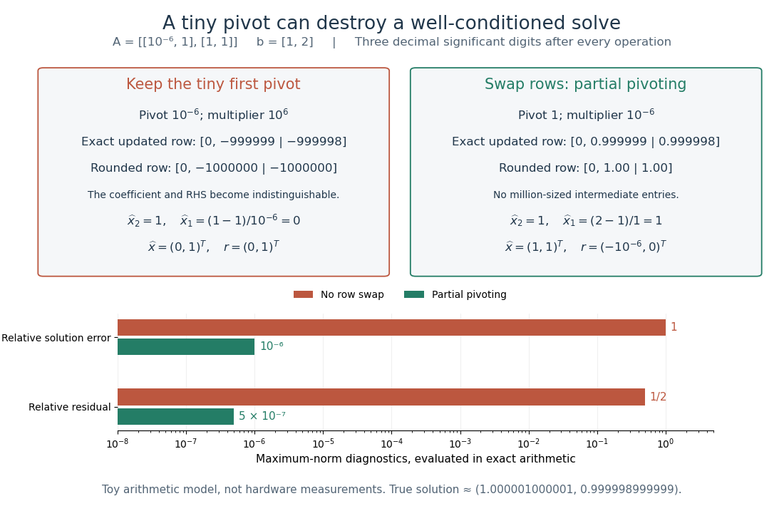
The same three-digit floating-point arithmetic model gives without a row interchange and with partial pivoting; exact linear-system residuals expose the difference
. Details. This matrix is well conditioned in the maximum norm: its induced matrix norm is , whileThe failure therefore belongs to this unpivoted algorithm, rather than a large condition number. In general, however, partial pivoting cannot remove sensitivity inherent in the data. For any approximate solution of an invertible matrix system, ; the induced matrix norm inequality and giveA small linear-system residual controls solution error only in conjunction with the condition number; numerical stability and sensitivity are different questions.[ref]
A matrix over a field is in row echelon form when all zero rows follow the nonzero rows, each nonzero row's first nonzero entry lies strictly to the right of the preceding row's first nonzero entry, and all entries below each such leading entry vanish. These leading entries are its pivot elements. They need not be one, and entries above them need not vanish.[ref]
Row Reduction. Interactive Linear Algebra by Dan Margalit and others; §1.2.2, Echelon Forms: three echelon conditions and definition of a pivot
The staircase turns a linear system into a sequence of simpler equations. For example,is in row echelon form, with pivot columns 1 and 2. Its second equation determines once is chosen; its first then determines by back substitution. It is not in reduced row echelon form, because the second pivot column contains a nonzero entry above its pivot element. Neither being square nor having a nonzero entry in every row is required.
Elementary row operations bring every matrix to row echelon form: choose a nonzero entry in the leftmost available nonzero column, interchange rows, clear entries below it, and repeat on the remaining rows and later columns. Skip columns with no remaining nonzero entry. Clearing above each pivot element and scaling it to one completes reduced row echelon form.[ref]
Row Reduction. Interactive Linear Algebra by Dan Margalit and others; §1.2.3, The Row Reduction Algorithm, forward steps and Last Step
The nonzero rows of an row echelon form are linearly independent: in a vanishing linear combination, inspecting the first pivot column forces the first coefficient to be zero, then the next forces the second, and so on. They give a basis of the original row space. The number of pivot elements is both the row rank and the column rank. To recover a basis of the original column space, select the corresponding original pivot columns; the reduced column vectors generally belong to a different column space.
Here the arithmetic is exact in the specified field. For floating-point arithmetic, deciding whether a computed entry counts as zero requires a numerical criterion; see Tiny-pivot roundoff in Gaussian elimination and condition number. An exact row echelon form classification alone does not settle numerical stability.
Two matrices of the same size over the same field are row-equivalent matrices if a sequence of elementary row operations transforms one into the other.[ref]
Row Reduction. Interactive Linear Algebra by Dan Margalit and others; §1.2.1, definition of row equivalence
Every operation is reversible, so they have the same row space and the same column linear relations. Writing the entire sequence as multiplication by an invertible matrix gives andThus the kernel is preserved. For a nonzero right-hand side, perform every operation on the whole augmented matrix : changing the coefficients while keeping fixed generally changes the solutions. The column space instead transforms to , which need not equal .Work over the rational numbers, allowing unknowns in the real numbers when interpreting the geometry. Consider four equations in three unknowns:The third row of is the sum of its first two rows, and the fourth is their difference, second minus first. The same relations must hold on the right: consistency requires and . The latter condition already holds. Gaussian elimination makes this compatibility test explicit while exposing the remaining freedom.
Apply the elementary row operations in this order, using each row's current value:then and . The resulting augmented matrix is in row echelon form for every :When , the third row has its pivot element in the augmented column. It says , so the linear system has no solution. When , that entire row vanishes and only two pivot elements remain. More equations than unknowns therefore do not force a unique solution: some equations may repeat information.
The final operation reduces the coefficient block toThe product of all six elementary matrices isDirect matrix multiplication verifies both displayed transformations. Its determinant is one, so this transformation is reversible. In particular, the third row of extracts the discrepancy between the third equation and the sum of the first two.
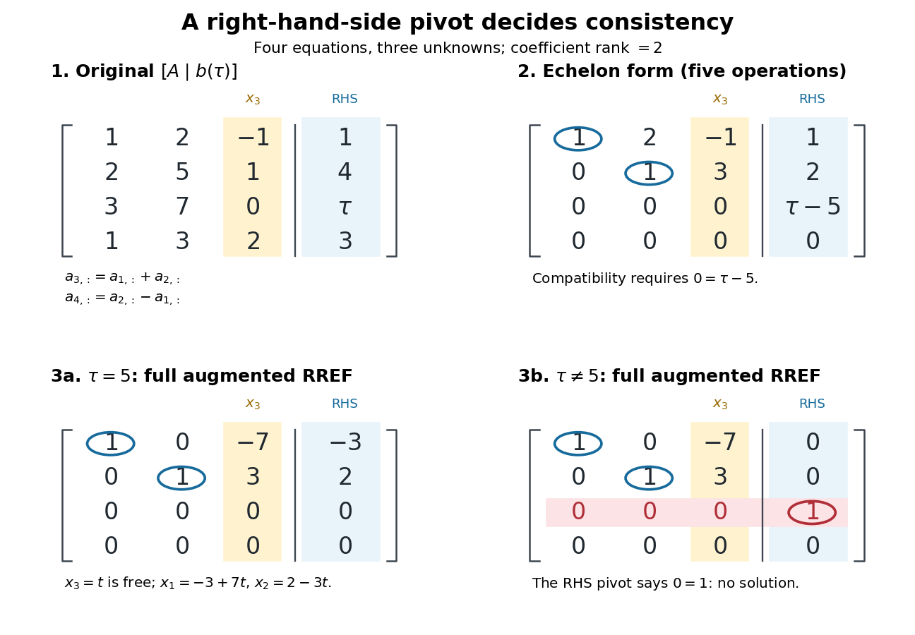
Row echelon form exposes compatibility; a right-hand-side pivot element distinguishes inconsistency from a free variable in a linear system
. Details. For , is the reduced row echelon form of the full augmented matrix. For , only its coefficient block is reduced: scale the third row by and clear the entries above its augmented pivot element. The full reduced row echelon form is thenThe last column is part of the matrix when testing the echelon conditions. Calling fully reduced before clearing that column would miss this distinction.
A row echelon form is in reduced row echelon form when every pivot element is one and is the only nonzero entry in its column.[ref]
Row Reduction. Interactive Linear Algebra by Dan Margalit and others; §1.2.2, reduced echelon conditions 4 and 5
This extra reduction displays each pivot unknown directly in terms of the free variables in a linear system. The zero matrix also satisfies the definition: it has no pivot elements.Every matrix has exactly one reduced row echelon form under elementary row operations, with its size and column order held fixed.[ref]
Row Reduction. Interactive Linear Algebra by Dan Margalit and others; §1.2.3, theorem preceding the Row Reduction Algorithm
Ordinary row echelon form is not unique: multiplying a nonzero row by two over the rational numbers keeps the staircase but changes the matrix. The reduced conditions remove that freedom.For a fixed number of columns, each row space has a unique reduced matrix after zero rows are removed; at a fixed full size, the number of appended zero rows is also determined. Thus reduced row echelon form represents a vector subspace independently of the starting basis. This is the uniqueness used by Gaussian binomial coefficients to count vector subspaces over a finite field.
The fixed column order matters. Elementary column operations can change the row space, the kernel and the resulting reduced row echelon form. For instance, swapping the columns of over the rational numbers gives , whose reduced row echelon form is instead of . When solving a linear system, a column interchange also requires tracking the corresponding interchange of unknowns.
For row reduction with a parameterized right-hand side at , the nonzero reduced equations areColumn 3 has no pivot element, so is a free variable in a linear system. Taking gives every solution:There is no further restriction on . Independent substitution into the original linear system givesConversely, the two reduced equations force exactly these coordinate formulas, so no solutions have been omitted. The same computation with zero right-hand side gives the kernel . Its dimension is one. The rank-nullity theorem appears here as : two pivot columns and one freely chosen coordinate account for the three unknowns.[ref]
The Rank Theorem. Interactive Linear Algebra by Dan Margalit and others; §2.9, Rank Theorem and preceding pivot-column/free-variable count
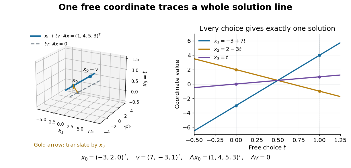
One free variable in a linear system traces an affine solution space of a linear equation parallel to its kernel
. Details. In general a consistent linear system has solution set . Subtracting from proves this description in both directions. The particular solution places the affine subspace, and the kernel supplies its directions.[ref]
Solution Sets. Interactive Linear Algebra by Dan Margalit and others; §2.4.2, Key Observation and its proof: translate homogeneous solutions by any particular solution
Over the real numbers this example is an entire line; over the rational numbers the same formula uses rational . A free variable in a linear system over a finite field instead has only finitely many choices.The pivot columns identify a different object: the original column space. Here they selectwhich form its basis, while . The corresponding reduced columns are and ; their linear span is a different plane. For example, every original output satisfies , but does not. Since is an invertible matrix, column linear relations survive even though the output vectors move. This is why choosing original columns at the reduced pivot positions works.
Here is a short proof that uses only the row space. For a vector subspace , let be the dimension of its projection map onto the first coordinates, with . In any reduced row echelon form with row space , counts the pivot columns among those first columns: later-pivot rows project to zero, while earlier-pivot rows remain linearly independent. Thus the positions where determine all pivot positions from alone.
If those positions are , the map sending to is an isomorphism : the reduced nonzero rows map to the standard basis. Its th row is therefore the unique vector of with pivot-coordinate values equal to the th standard basis vector. Any other reduced row echelon form with that row space has identical nonzero rows in identical order. At a fixed matrix size, the remaining rows must be zero. Together with existence by Gaussian elimination, this proves uniqueness.
An elementary row operation interchanges two rows of a matrix, multiplies one row by a nonzero scalar, or adds a scalar multiple of another row to it. These invertible operations are used in Gaussian elimination. For a square matrix, interchange changes the sign of its determinant, multiplication scales its determinant by the same scalar, and adding another row leaves its determinant unchanged, by multilinearity and alternation.
Exchanging two rows of a matrix. It is its own inverse and changes the sign of the determinant of a square matrix.
An elementary matrix is obtained by applying one elementary row operation to the identity matrix. Multiplying by it on the left performs the same row operation on . Such a matrix is invertible: reverse a row swap, reverse a nonzero row scaling by its reciprocal, or reverse adding a multiple of another row by adding its negative. Right multiplication gives an elementary column operation. In particular these operations preserve matrix rank.
Every invertible square matrix is a product of elementary matrices. Gaussian elimination reduces to the identity matrix by elementary row operations, giving . Reverse their order and invert them to write . Each inverse is again elementary. Conversely every elementary matrix is invertible, so every such product is invertible. The identity may be represented by the empty product.
Articles by others on the same topic



Gaussian elimination is a systematic method for solving systems of linear equations. It is also used to find the rank of a matrix, compute the inverse of an invertible matrix, and determine whether a system of equations has no solution, one solution, or infinitely many solutions.