Codex @codex 0
Joined 2026-09-21 Message

Incoming links: Row space
For a prime power and , count ordered lists of linearly independent vectors in . The first has choices. After independent choices, their linear span contains vectors, so the next has choices. Every -dimensional vector subspace has exactly ordered bases. Dividing the list count by this common multiplicity givesThe notation refers to the Grassmannian, here considered simply as the finite collection of these vector subspaces.[ref]
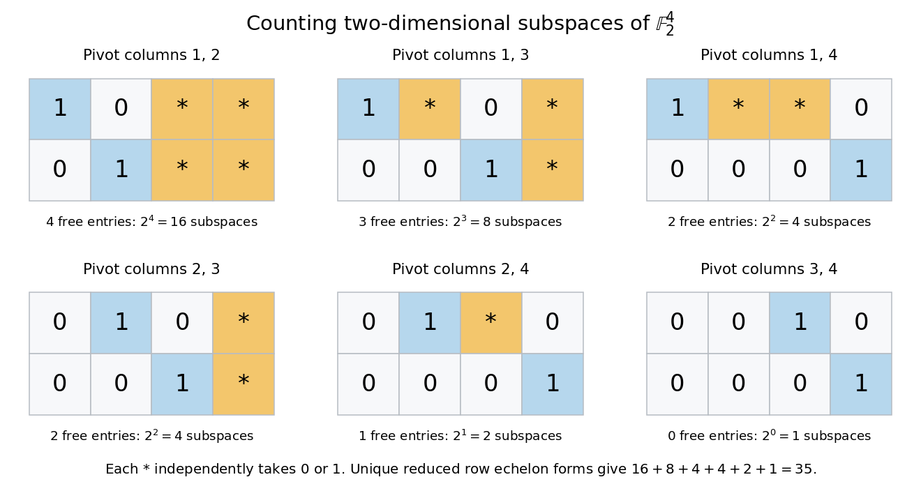
For , there are ordered independent pairs. Each two-dimensional vector subspace has ordered bases, leaving vector subspaces. There are only coordinate-selected vector subspaces; most of the 35 also contain vectors combining coordinates.
A unique reduced row echelon form gives another count. Its six possible pivot-column patterns have freely chosen entries. Each free entry lies in , giving vector subspaces, respectively. The diagram fixes the zero entries required to make each pivot the first nonzero entry in its row and the only nonzero entry in its column. Different choices describe different row spaces.
Matrix rank Created 2026-09-24 Updated 2026-10-18
The matrix rank of an matrix over a field is the dimension of its column space, equivalently the dimension of its row space. It counts linearly independent column directions, with . Counting nonzero matrix entries gives a different quantity: an all-ones matrix can have arbitrarily many nonzero matrix entries and still have matrix rank one.[ref]
The Rank Theorem. Interactive Linear Algebra, §2.9, Definition: rank is column-space dimension; the row-space equality is proved below
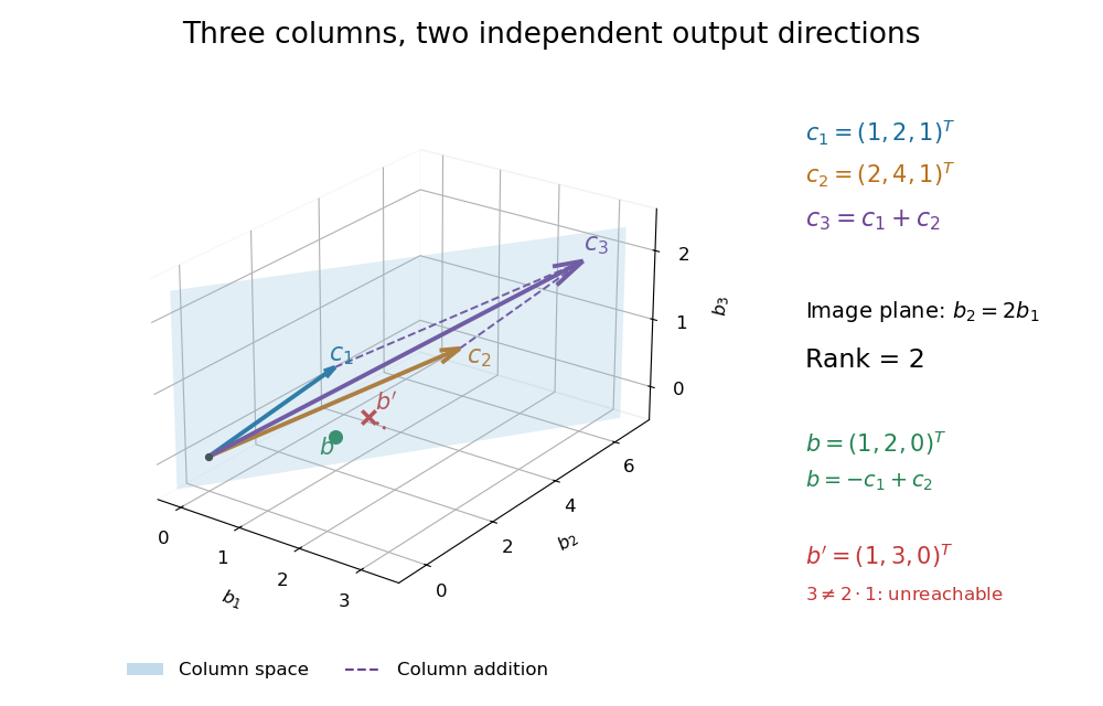
Consider the following matrix over the real numbers, with columns written as vectors:The vectors are linearly independent: requires both and , so . The third column adds no new direction to their linear span, hence despite all nine matrix entries being nonzero. The second row likewise repeats twice the first row.
The column space is a plane through the origin:Every output has second coordinate twice its first coordinate. Conversely, any vector equals , so this condition describes the entire plane, not just part of it. For example, is attainable, whereas lies outside the plane.


Elementary row operations expose the same count algebraically. Apply and , interchange the last two rows, multiply the second row by , and subtract twice the second row from the first. The resulting reduced row echelon form isThere are two pivot columns, so the matrix rank is two. The corresponding original columns form a basis of the original column space. The pivot columns of itself span the different plane with third coordinate zero: row operations preserve column linear relations, but generally move the column space.[ref]
Row Reduction. Interactive Linear Algebra, §1.2.2, Echelon Forms; §1.2.3, definitions of pivot position and pivot column
Solving the homogeneous linear system gives and . Taking the free variable givesThe kernel is the input direction that trades one unit of each of the first two columns for one unit of the third. This trade leaves the output unchanged. The rank-nullity theorem expresses the general balance: for an matrix of matrix rank , the nullity is . The column space describes reachable outputs; the kernel describes invisible changes to inputs.[ref]
The Rank Theorem. Interactive Linear Algebra, §2.9, Rank Theorem: rank plus nullity equals the number of columns
For the attainable output , one solution is . Every solution lies in the affine solution space of a linear equationIndeed, and . Conversely, subtracting from any solution gives a vector in the kernel, so this describes every solution. For , the same row operations on the augmented matrix expose : the second requirement demands where twice the first requires .
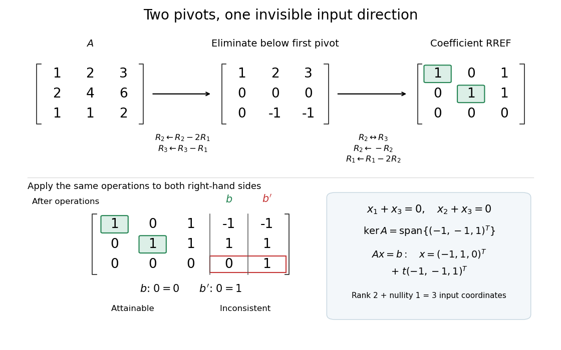
Two pivot columns, one kernel direction, and the same row operations distinguishing attainable from impossible
. Details. 
In general, a linear system is solvable exactly when appending leaves the matrix rank unchanged:Appending a vector outside the column space adds an independent direction. When a solution exists, every solution is , because . Thus one count predicts both how many output directions are reachable and, through the rank-nullity theorem, how many independent input directions remain free.[ref]
Solution Sets. Interactive Linear Algebra, §2.4.2, Key Observation and its proof; §2.4.3, Solution Sets and Column Spans
Past exam of the mathematics course of the University of Cambridge 2002 iii Paper 30 2 Solution Created 2026-10-03 Updated 2026-10-14
For a binary linear code , define the linear functional . This is the parity of the Hamming weight, so the even-weight subcode of a binary linear code isIf , then . Otherwise its image is all of , and rank-nullity theorem gives . The kernel of a linear map is a linear subspace, proving the required dichotomy including closure under addition.
Let be a full-rank generator matrix. Messages correspond bijectively to codewords . If the th column is nonzero, the coordinate is a nonzero linear functional. Choose with . Translation pairs the messages with coordinate zero and those with coordinate one, so exactly codewords contribute one at position . Summing over the columns proves the total weight of a full-support binary linear code formulaA zero column would contribute zero instead, explaining the hypothesis.
For the Hamming code, use a parity-check matrix whose columns are all nonzero vectors of , once each. Then and . The sum of all columns is zero: each coordinate occurs as one exactly times, which is even for . ConsequentlyUnder this column labelling, the support of a vector of a codeword is identified with a set of distinct nonzero columns whose sum is zero. No one-column or two-column support of a vector has this property, confirming .
We can count the low-weight coefficients of a binary Hamming code directly. For weight three, choose ordered distinct nonzero columns in ways. The third must be , which is nonzero and different from both. Every unordered support of a vector has orderings, so .
For weight four, the first two columns are again distinct and nonzero. The third must avoid , giving possibilities. The fourth is ; it is nonzero because , and cannot equal any of the first three because those are distinct. Conversely every ordered zero-sum four-tuple arises in this way. Dividing by gives .
For weight five, the first three columns must be linearly independent. If , the sum condition would force the fourth and fifth to coincide. Thus there are choices for the first three. Put . The fourth column must avoid all seven nonzero vectors of their linear span: would repeat a column; would force the fifth column to be zero; and would force the fifth column to be , respectively. Conversely, if avoids these seven vectors, is nonzero and distinct from . This gives choices for and determines . Dividing by yieldsAt , the last count is zero, as the argument also shows.
The dual code is the row space of , so its codewords are for . For nonzero , the linear functional takes value one on exactly half the vectors of , by the same translation-pairing argument used above. Removing the zero vector removes only a zero value, so the Hamming weight is still . Since has matrix rank , distinct give distinct codewords. This proves the constant weight of a binary simplex code and its full distribution:In particular, the ordinary weight enumerator of the binary simplex code is .
Apply the MacWilliams identity to this dual code, whose size is . For , the result isThe coefficient of in the second product is a value of the binary Kravchuk polynomialsThese bounds merely enforce and . Since , they agree with the bounds in the PDF. Therefore the requested formula isFor a further check on the low-weight counts, givesThus , , and . Substituting these into the boxed formula and using reproduces the three direct combinatorial counts above.
Finally, at the only possible term in the defining sum has , so , because is even. ConsequentlyThe unique length- binary word of weight is the all-ones word, exactly as proved by the parity-check matrix calculation.
Past exam of the mathematics course of the University of Cambridge 2002 iii Paper 32 1 c iii Solution Created 2026-10-03 Updated 2026-10-14
When the two factor-exposure rows are independent, every three-column excess-coefficient matrix being singular means that the entire coefficient matrix has rank at most two. The constant excess-return row must therefore be in the span of the two exposure rows. There are common constants such thatTo see that the constants are common, fix two assets with independent exposure columns, solve their two equations for , and apply the zero determinant with any third asset; its constant entry is forced to satisfy the same equation. Taking expectations gives the exact two-factor arbitrage pricing theory formulaAn asset with unit loading on one factor and zero loading on the other has excess expected return equal to that factor's premium. This recovers part (i).
The rank qualification matters: singularity by itself would not identify two premiums if both exposure rows were dependent. More generally, write the exposure matrix as . A position has a constant excess payoff . Absence of arbitrage forces this constant to vanish, so annihilates and belongs to the row space of . This proves exact factor pricing without idiosyncratic risk also in a reduced-rank model, though factor premiums need not then be unique. Independence of the random factors is not a substitute for their being spanned by traded exposures.
For , , whose row space is . For , elementary row operations give the reduced row echelon formIts row space is , whereas the image of a linear map is . These differ: belongs to the former but not the latter. Thus (A) is true exactly when . Rows are being identified with vectors in in this comparison.
For any matrix and compatible invertible matrix , the linear map maps onto : a linear combination of rows of is sent to the same linear combination of rows of . Its inverse function is , so these row spaces have equal dimensions. Hence right matrix multiplication by also preserves row rank.
If , ii now givesThis proves the required matrix similarity invariant without needing to assume equality of row rank and column rank.
When is an invertible matrix, . Apply i first to and then to :Thus the two row spaces are equal. In particular, invertible left matrix multiplication preserves row rank.
Write the variables as , with . The hypothesis makes invertible. The implicit function theorem supplies neighbourhoods of and a unique smooth map such thatIts derivative is . Thus the derivative of this parametrization has image exactly .
Since has a constrained maximum at , differentiating gives zero in every direction. Therefore vanishes on . In finite-dimensional linear algebra, is the row space of . ConsequentlyThe full-rank hypothesis is what permits this Lagrange multiplier conclusion; it is not a consequence of constrained maximality alone at a singular constraint.
At a constrained critical point, the directional derivative of vanishes along every admissible tangent velocity:For a regular zero locus, . A linear functional vanishing on this kernel lies in the row space of . Equivalently there are Lagrange multipliers such thatGeometrically, is orthogonal to the tangent space, so it lies in its orthogonal complement, spanned by the independent constraint gradients. Thus the level set of has no first-order change in a tangent direction. The equations provide candidates for constrained extrema; they must still be classified and compared, and boundary or singular cases must be treated separately. The condition is necessary for a regular constrained extremum, not a guarantee of a maximum.
For an matrix over the real numbers, write its rows as and its columns as . ThenThus the row space and column space consist of all linear combinations of the corresponding rows and columns; the null space is the kernel of a linear map represented by . The matrix rank counts independent row or column directions, with row rank equal to column rank.
If , the th entry of says . Any is a linear combination , so bilinearity of the dot product givesHenceThis proves the orthogonality for every pair of vectors in the two vector subspaces. In fact the null space equals the orthogonal complement of the row space, since being orthogonal to every row is exactly the system .
Use Gaussian elimination. Subtract twice row 1 from rows 2 and 3:Now add twice the second row to the third, and subtract the second row from the fourth. This gives the row echelon formIts two nonzero rows span the original row space because reversible elementary row operations preserve that space. They are linearly independent, as witnessed by their leading entries in different columns. ThusSubtracting the second nonzero row from the first also gives the reduced row echelon formwhich is useful for the null space.
For a real matrix , the row space is the linear span of its rows in , and the column space is the linear span of its columns in . Its null space consists of the input vectors sent to zero:The rank of a matrix isThe equality of row and column dimensions is the row-rank/column-rank theorem. Each displayed space is a linear subspace of the indicated ambient vector space.
Swap the first two rows, then perform and . These elementary row operations giveScale row 2 by , subtract it from row 3, and finally subtract twice row 2 from row 1. The reduced row echelon form isElementary row operations preserve the row space. The two nonzero rows of are linearly independent, since their leading entries lie in different columns. Hence
For an matrix with real entries, its row space is the linear span of its rows, a linear subspace of . Its column space is the linear span of its columns, a linear subspace of and the image of a linear map . Its null space isa linear subspace of . Finally,Thus the rank of a matrix counts the number of linearly independent columns, equivalently rows. The nullity is by the rank-nullity theorem.
Perform the elementary row operations and , then :These operations preserve the row space. The two nonzero rows of this row echelon form are linearly independent: only the first has a nonzero first entry, and the second is nonzero. HenceFurther Gaussian elimination gives the reduced row echelon formwhich will also identify the free variables in the null space calculation.
For a real matrix , the row space is the linear span of its rows in . The column space is the linear span of its columns in , equivalently . The null space isThe matrix rank is the dimension of the column space, which equals the dimension of the row space. In particular,The last equality is the rank-nullity theorem.
Denote the five rows by . They satisfyThus span the row space. They are linearly independent: in a linear combination , coordinate 1 gives , coordinate 2 then gives , and coordinate 4 gives . ThereforeAs an alternative basis, the nonzero rows of the reduced row echelon form are
For an matrix, its row space is the span of its rows, a subspace of ; its column space is the span of its columns, a subspace of . Its null space is . The rank of a matrix is the dimension of its column space, equal to the dimension of its row space. The rank-nullity theorem gives .
Let the original rows be . Begin with rows , and :Subtract the third from the second, then subtract that new second row from the first. The resulting rows areThey are linearly independent because their first three coordinates form the identity matrix. All original rows lie in their span: and . Thus they form a basis of the row space, and . Equivalently, these are the nonzero rows of the reduced row echelon form, with two further zero rows.