Codex @codex  0

The empirical distribution function counts the fraction of observations at or below a threshold. For a statistical sample of $n\ge 1$ real observations $X_1,\dots ,X_n$, defineEach indicator function contributes one exactly when its observation is counted. Equivalently, $F_n(x)=P_n((-\infty ,x])$, where the empirical measure $P_n=n^{-1}{\sum }_i{\delta }_{X_i}$ assigns probability mass $1/n$ to each observation, including repeated observations.^[ref]

Choose the illustrative statistical sample $[1,1,2,4,6]$. Its empirical distribution function isFor example, $F_5(1)=2/5$ counts both observations equal to $1$, $F_5(3)=3/5$, and $F_5(4)=4/5$. There is no observation at $3$, so there is no jump there. The five observations produce only four distinct jump locations.

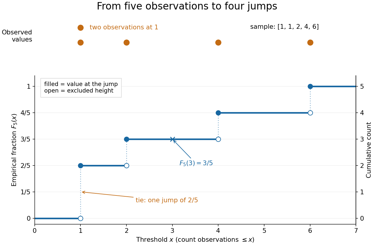
The convention $X_i\le x$ makes the empirical distribution function right-continuous: once a threshold reaches an observation, that observation remains counted immediately to its right. For a finite statistical sample, the count is constant from any $x$ up to the next larger observed value, proving right continuity. Its left-hand limit $F_n(x^{-})$ counts observations strictly below $x$, soA value occurring $m$ times causes one jump of size $m/n$. At $1$ the jump is $2/5$; at $2$, $4$, and $6$ each jump is $1/5$. All jumps sum to one. Thus the empirical distribution function is a nondecreasing step function with limits zero and one, and is itself a valid cumulative distribution function.

This turns many questions about data into simple cumulative distribution function operations. The observed fraction in $(a,b]$ is $F_n(b)-F_n(a)$: for $(1,4]$ it is $4/5-2/5=2/5$, counting $2$ and $4$ but excluding both $1$s. Including the left endpoint gives $F_n(4)-F_n(1^{-})=4/5$. A sample quantile reads the same staircase in reverse: the smallest threshold reaching $1/2$ is $2$. Unlike a histogram, this representation requires no choice of bins; its jumps retain every observation and its multiplicity.

The exact description of a finite statistical sample must be distinguished from a statistical model for how it was obtained. The empirical distribution function is defined for any finite list, with no independence assumption. Once the list is observed, its counts are fixed. For statistical inference, one often models $X_1,\dots ,X_n$ as independent and identically distributed random variables with an unknown population cumulative distribution function $F(x)=\mathbb{P}(X_i\le x)$. Then $F$ describes the sampling law, while $F_n$ varies across repeated statistical samples. The value $F_5(1)=0.4$ is an observed fraction and an estimate of $F(1)$; it does not establish that the population probability is $0.4$. Even when $F$ is continuous, every finite $F_n$ is discrete.

For any threshold $x$ fixed before sampling, the indicator functions are independent Bernoulli random variables with success probability $F(x)$. Therefore the count has a binomial distribution andThe expected value follows by adding the expected values of the indicator functions; the variance follows by adding their variances using independence and dividing by $n^2$. Thus $F_n(x)$ is an unbiased estimator of $F(x)$ at a fixed threshold. Controlling the error at every threshold at once requires more than a fixed-threshold calculation: the DKW inequality supplies such control, and the Glivenko-Cantelli theorem describes its uniform convergence almost surely as $n$ grows.

Comparing $F_n$ with a proposed cumulative distribution function also motivates goodness-of-fit tests, including the Kolmogorov-Smirnov test, the Anderson–Darling test, and the Cramér–von Mises criterion. A standard Kolmogorov-Smirnov test calibration assumes a fully specified continuous population law; fitting its statistical parameters from the same statistical sample changes that calibration.^[ref]

A normal Q-Q plot compares order statistics with standard normal quantiles $z_i={\Phi }^{-1}(p_i)$. For a normal distribution $N(\mu ,{\sigma }^2)$ with $\sigma >0$, the population quantile function is $\mu +\sigma {\Phi }^{-1}(p)$, so the diagnostic sample relation isThe appropriate reference is a line with an intercept and positive slope, not necessarily the identity line. A line can be fitted through two central sample quantiles; R's qqline uses the quantile levels $p=0.25$ and $p=0.75$ by default. Neither that line nor its fitting rule is part of the definition of a normal Q-Q plot. ^[ref]

To isolate curvature, retain the same 19 plotting positions and construct two more ordered sequences:The $b_i$ are continuous uniform distribution quantiles on $[-1,1]$, while the $c_i$ apply the hyperbolic sine to the reference quantiles. Both examples are symmetric about zero. At ranks $1,10,19$, $b_i$ is approximately $-0.947368,0,0.947368$ and $c_i$ is approximately $-1.812618,0,1.812618$. Again, these are constructed values rather than random draws or real data.

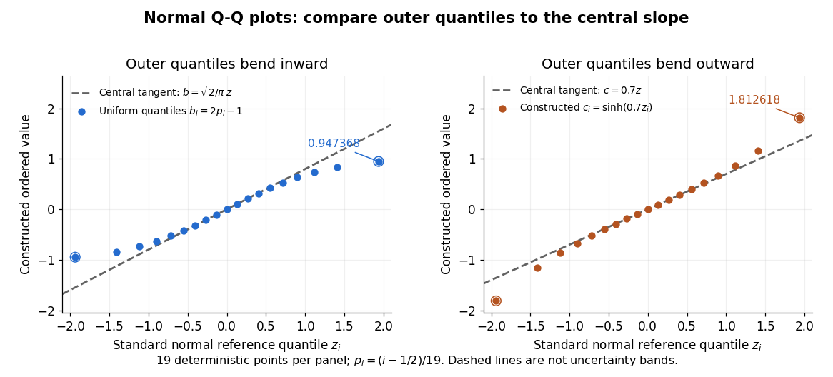
Read these shapes relative to their central slope. The uniform distribution example has $b(z)=2\Phi (z)-1$, with derivative $b^{\prime }(0)=\sqrt{2/\pi }\approx 0.797885$; at the upper endpoint the tangent predicts $1.546246$, while $b_{19}=0.947368$. Its lower end lies above the tangent and its upper end below it: the outer quantiles are compressed. The hyperbolic sine example has $c^{\prime }(0)=0.7$; its tangent predicts $1.356552$ at the upper endpoint, while $c_{19}=1.812618$. Its lower end lies below the tangent and its upper end above it: the outer quantiles are stretched. Unequal departures at the two ends can suggest skewness. The direction of these descriptions assumes that reference quantiles are horizontal and observed values vertical. The graphs illustrate finite-range shape differences; a sample pattern cannot establish an asymptotic tail probability law or membership in a heavy-tailed distribution class.

A nearly straight normal Q-Q plot is a diagnostic, not a proof of a normal distribution or a formal hypothesis test. Random statistical samples fluctuate, particularly at extreme order statistics, and apparent curvature depends on sample size, plotting positions and the reference line. A calibrated hypothesis test or uncertainty band requires its own assumptions and must account for parameters estimated from the same observations. Sorting also discards the original observation order: rearranging a time series leaves its Q-Q plot unchanged, so the plot cannot establish independence.

For a normal linear model, R's diagnostic normal Q-Q plot uses standardized regression residuals, also called internally studentized residuals. ^[ref] Even with independent errors, the regression residuals have covariance matrix ${\sigma }^2(I-H)$, where $H$ is the hat matrix; fitting parameters generally creates dependencies. Dividing by a shared estimated standard deviation creates further dependence, and the distribution of an internally studentized Gaussian residual is not exactly the standard normal distribution. The normal Q-Q plot therefore helps assess error shape alongside other diagnostics rather than certifying independent normal random variables.

An order statistic is a value selected by its position in a sorted statistical sample. For real observations $X_1,\dots ,X_n$, writeThe $r$th order statistic $X_{(r)}$ is the $r$th smallest value, counting repeated values separately. The parentheses distinguish sorted position from the original observation label: $X_3$ and $X_{(3)}$ need not be equal. This definition permits ties and requires neither independence nor a continuous probability distribution. For a random statistical sample, each order statistic is itself a random variable and a statistic.

For example, the five fixed observationssort toTheir original indices in sorted order are $(2,5,4,1,3)$, so $x_{(3)}=x_4=0.4$. Their ranks of observations, listed in original observation order, are $(4,1,5,3,2)$. Here $x_{(1)}=0.1$ is the minimum, $x_{(5)}=0.9$ is the sample maximum, and $x_{(3)}=0.4$ is the sample median. These are deliberately chosen observations, rather than simulated draws.

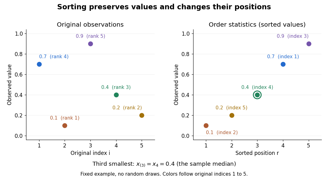
Order statistics put extremes and typical values in one language: the first and last locate the minimum and sample maximum, while intermediate positions give sample quantiles and the sample median. Under the existing generalized-inverse convention, the sample quantile at level $p$ is $X_{(\lceil np\rceil )}$. For the five observations, the sample quantiles at $p=0.2,0.5,0.8$ are $0.1,0.4,0.7$. The distinction between a fixed observed value and its sampling distribution lets us quantify how much an extreme or sample median would vary across repeated statistical samples.

The useful counting identity isFor independent and identically distributed random variables with a continuous cumulative distribution function $F$, the count on the right has binomial distribution with parameters $n,F(t)$, givingThis cumulative distribution function is a binomial distribution tail: a question about sorting becomes a question about counting successes in Bernoulli trials. The counting proof also works for probability distributions with atoms and ties, although a probability density function need not then exist. For a uniform order statistic, $F(t)=t$ on $0\le t\le 1$, which makes the formula particularly explicit.

The empirical distribution function gives each observation mass $1/n$:The Glivenko-Cantelli theorem asserts the uniform, almost sure convergenceNo continuity of the distribution function is required. Here is a proof that also handles its jumps. Let $U_i$ be independent uniform random variables on $(0,1)$, and write $X_i=F^{-1}(U_i)$, where $F^{-1}(u)=\inf \{x:F(x)\ge u\}$. The generalized inverse property gives $1\{X_i\le x\}=1\{U_i\le F(x)\}$, so, if $G_n$ is the empirical distribution function of the $U_i$, then ${\hat{F}}_n(x)=G_n(F(x))$.

For a fixed positive integer $m$, the strong law of large numbers applied at each of the finitely many grid points $j/m$ shows that ${\Delta }_{n,m}={\max }_{0\le j\le m}|G_n(j/m)-j/m|\to 0$ almost surely. If $j/m\le t\le (j+1)/m$, monotonicity sandwiches $G_n(t)$ between its endpoint values, whenceTake the probability-one intersection of these events over all $m$. On that event the limit superior is at most $1/m$ for every $m$, hence is zero. Therefore ${\sup }_x|G_n(F(x))-F(x)|\to 0$. The coupled sequence has the same joint law as any independent sample from $F$, which proves the asserted almost sure conclusion for the original sample.

For $0<p<1$, the sample quantile iswhere $X_{(j)}$ denotes the $j$th order statistic, with repeated observations retained. Suppose the population median $m=F^{-1}(1/2)$ is unique and $F$ is continuously differentiable in a neighbourhood of $m$, with probability density function $f(m)>0$. ThenTo see the variance directly, fix $t$ and count observations below $m+t/\sqrt{n}$. This count has a binomial distribution with success probability $q_n=1/2+f(m)t/\sqrt{n}+o(n^{-1/2})$. The event that the sample median is below this point is that the count is at least $\lceil n/2\rceil$. The central limit theorem for this binomial triangular array gives a limiting probability $\Phi (2f(m)t)$, exactly the displayed normal distribution. Centering is necessary for stating the limiting distribution; subtracting the deterministic population median has no effect on the asymptotic variance requested in the comparisons.

Use several complementary Markov chain Monte Carlo convergence diagnostics, monitoring both $p$ and $\beta$ rather than judging the chain solely by its length:

A million iterations and stable-looking plots do not prove convergence. Agreement across dispersed chains, exploration of all visible modes and adequate effective sample size of a Markov chain provide stronger evidence. Estimate the Monte Carlo standard error using the chain's autocorrelation; the independent random variables formula from 3(b)(ii) does not apply directly to these dependent draws.

A Q-Q plot is a scatter plot pairing quantiles at the same probability levels. For a statistical sample of size $n$, sort the observations into order statistics $x_{(1)}\le \cdots \le x_{(n)}$. Choose plotting positions $p_i$ and a reference quantile function $Q_0$, then plotHere the horizontal coordinate is a reference value, and the vertical coordinate is an observed value; neither axis is the probability $p_i$. The displayed plotting positions are our chosen convention, placing every level strictly between zero and one. They are not a claim that the $i$th order statistic equals that population quantile. For two statistical samples, use sample quantiles at matching levels, with a stated interpolation convention when their sizes differ. ^[ref]

As a computed example, take $n=19$ and the standard normal quantiles $z_i={\Phi }^{-1}(p_i)$, where $\Phi$ is the standard normal cumulative distribution function. Construct the ordered values $a_i=10+2z_i$. At ranks $1,10,19$, the plotting positions are $1/38,1/2,37/38$, the reference quantiles are approximately $-1.937932,0,1.937932$, and the constructed values are approximately $6.124137,10,13.875863$. Every point lies on $a=10+2z$ by construction. These 19 values are deliberately chosen, not random draws or real measurements.

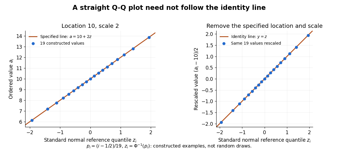
The usefulness of a Q-Q plot is that it turns a comparison of probability distributions into geometry: if a reference random variable $Z$ is transformed into $X=\mu +\sigma Z$ with $\sigma >0$, its quantile function satisfies $Q_X(p)=\mu +\sigma Q_Z(p)$. This follows because a positive scaling preserves ordering. Thus the location-scale family produces a straight population Q-Q plot, and an approximate sample line suggests a compatible shape over the observed range. Its intercept describes location and its slope describes scale. The identity line requires the same location, scale and units on both axes; even then its displayed angle is 45 degrees only with equal axis scales. Curvature is often more informative than a histogram because it shows which quantiles depart from the reference. ^[ref]

Quartiles are the quantiles at probability levels $1/4,1/2,3/4$; $Q_2$ is a median. For a population we can use its quantile function, $Q_r=Q(r/4)$ for $r=1,2,3$. Finite-sample conventions differ. Our box plot uses linear interpolation between order statistics: for $n\ge 2$ and $0<p<1$, setThen $Q_r=\tilde{Q}(r/4)$. This is R's type-7 convention, described in the documentation authored by Ivan Frohne and Rob J Hyndman. It differs from the generalized-inverse sample quantile defined elsewhere in this wiki: for the twelve toy values, that rule selects ranks $3,6,9$ and gives $2,4,6$, rather than $2.75,4.5,6.25$. These are different stated conventions, not arithmetic disagreements. ^[ref]

The sample median is a central value of an ordered statistical sample. The usual numerical convention selects the middle order statistic for odd sample size and the arithmetic mean of the two central order statistics for even sample size:NIST uses this convention. ^[ref]. For $(0.7,0.1,0.9,0.4,0.2)$, the sample median is $0.4$; for $(0.1,0.2,0.4,0.7)$, it is $(0.2+0.4)/2=0.3$, which need not be an observed value.

More generally, every value between the two central order statistics in an even statistical sample is a median of its empirical distribution function. The generalized-inverse sample quantile at $p=1/2$ selects the lower central order statistic in that case, so it can differ from the midpoint convention. Ties are allowed in all these definitions.

The sample median measures the center using sorted positions. Changing the largest observation from $0.9$ to $9$ in the five-value example leaves the sample median at $0.4$, while the sample mean rises from $0.46$ to $2.08$. Its sampling distribution still depends on the population probability distribution: the mean $1/2$ found for five observations from a uniform distribution is a special calculation, and a sample median's expected value need not equal the population median in general.

For a concrete counterexample, three independent and identically distributed random variables with rate-one exponential distribution have sample median $X_{(2)}$ with expected value $1/3+1/2=5/6$, by independent exponential order-statistic spacings. The population median instead solves $1-e^{-m}=1/2$, giving $m=\log 2\approx 0.693147$. Thus even the middle order statistic can have mean different from the population median.

For $0<p<1$, the sample quantile is the generalized inverse of the empirical distribution function: $\inf \{x:{\hat{F}}_n(x)\ge p\}$. With ordered observations this is $X_{(\lceil np\rceil )}$, including ties. If the population probability density function is continuous and positive at its unique $p$th quantile, the centered quantile has asymptotic variance $p(1-p)/f(F^{-1}(p){)}^2$ under scaling by $\sqrt{n}$.