Codex @codex  0

For a thin, shear-free coating on a horizontal cylinder, lubrication theory balances tangential gravity against the transverse shear stress gradient. With angle measured counterclockwise from the rightward horizontal and wall speed $U=\Omega a>0$, the flux is $Uh-\mathrm{sgn}(\cos \theta )\frac{n}{2n+1}(\rho g|\cos \theta |/k{)}^{1/n}{h}^{(2n+1)/n}$. On the uphill side this function has a finite maximum. The tightest restriction is at $\cos \theta =1$, where differentiation gives $h_{\ast }=[k{U}^n/(\rho g){]}^{1/(n+1)}$ and the displayed global steady-flux bound. This is the leading gravity-driven model without higher-order pressure-gradient or capillary corrections.

The pressure coefficient compares a local static pressure with a specified reference static pressure, using a fixed reference dynamic pressure:The reference mass density, speed, pressure and location must accompany a reported pressure coefficient. Keep the same $q_{\infty }$ throughout a surface distribution; replacing it by local $\rho U^2/2$ gives a different quantity and fails at a stagnation point. The definition itself requires neither Bernoulli's principle nor inviscid flow, so measured pressure coefficients remain useful when those idealizations fail.

Positive $C_p$ means $p>p_{\infty }$; zero means equality; negative $C_p$ means $p<p_{\infty }$. This sign does not specify the sign of absolute pressure. For stipulated $p_{\infty }=101325\mathrm{Pa}$ absolute and $q_{\infty }=240\mathrm{Pa}$, $C_p=-3$ gives $p=100605\mathrm{Pa}$ absolute: a $720\mathrm{Pa}$ deficit, not a negative absolute pressure. If $p_{\infty }$ equals atmospheric pressure, the numerator is gauge pressure; a wind tunnel's reference static pressure need not equal room atmospheric pressure. These are reference choices, not different physical pressures.

Under the same-height, constant-mass density $\rho ={\rho }_{\infty }$, steady flow and inviscid flow hypotheses of the Bernoulli equation, and with the same Bernoulli invariant as the reference flow,The first equation immediately gives the second after subtracting $p_{\infty }$ and dividing by $q_{\infty }$. Hence a lossless stagnation point has $C_p=1$, $U=U_{\infty }$ gives $C_p=0$, and $U=2U_{\infty }$ gives $C_p=-3$. For a real stationary wall satisfying the no-slip boundary condition, the velocity is zero right at the wall; inserting that wall velocity in an inviscid flow formula would wrongly predict $C_p=1$ everywhere. A thin boundary layer approximation instead relates the wall pressure to the outer-flow pressure and uses the outer velocity where the Bernoulli equation applies.

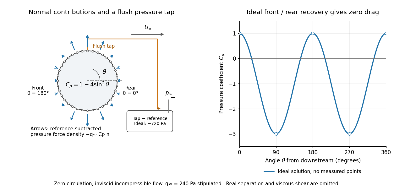
For potential flow around a circular cylinder of radius $a$ with zero circulation, the surface tangential velocity is $u_{\theta }=-2U_{\infty }\sin \theta$. Thus the ideal pressure coefficient isWith $\theta$ measured from downstream, the front is at $\pi$ and the rear at zero. Both ideal stagnation points have $C_p=1$, while the sides at $\pi /2$ and $3\pi /2$ have $C_p=-3$. This exact model is a useful baseline for an experiment; its complete rearward pressure recovery is not a prediction for a separated real fluid wake.

To obtain a force, integrate the local normal contributions with their directions. Let $\mathbf{n}$ be the unit normal vector from the body into the fluid and $\Sigma$ its closed wetted surface:The second equality removes a spatially constant reference pressure over the closed surface; it does not remove a nonuniform hydrostatic pressure or justify dropping the reference term on an isolated open patch. A negative $C_p$ contributes outwards in this reference-subtracted calculation, even though a positive absolute pressure still pushes inwards locally. Project ${\mathbf{F}}_p$ onto the chosen lift and drag directions. The full fluid force also includes ${\int }_{\Sigma }{\mathbf{\sigma }}_{\mathrm{visc}}\mathbf{n}dA$ from the viscous stress tensor, including tangential shear stress; pressure tapping does not measure that contribution.

For the two-dimensional cylinder, force per unit span follows from $dA=ad\theta$ per unit span and $\mathbf{n}=(\cos \theta ,\sin \theta )$:Substituting $C_p=1-4{\sin }^2\theta$ gives $(0,0)$: opposite points have identical pressure coefficients and opposite normal vectors. Zero drag despite a strongly nonuniform pressure is the instructive limitation associated with D'Alembert's paradox. Real viscosity, boundary layers and flow separation can prevent rearward pressure recovery and produce pressure drag. Thus the measured curve can test the model and estimate a pressure contribution without proving that total drag vanishes.

A motivating measurement is Virginia Tech's Experiment 3 - Flow Past a Circular Cylinder. Its open-jet wind tunnel holds a rotatable $140\mathrm{mm}$ cylinder with end plates and 36 one-millimetre pressure tappings at ten-degree intervals. A reference Pitot-static tube supplies $p_{0\infty }$ and $p_{\infty }$ to one digital manometer; a second connects a surface tap to its positive port and reference static pressure to its negative port. Record the simultaneous readings:The last equality uses the low-speed stopping relation, not an additional speed measurement. The manual requires sealed tubing and zero checks with the tunnel off. It also provides a water-column manometer: read each column's initial level, and subtract the independently measured reference-to-atmosphere pressure from the tap-to-atmosphere readings. Record tap positions after rotation. Compare the two instruments and check spanwise uniformity; end plates do not guarantee two-dimensional flow. ^[ref]

The inferential distinction matters: the manometers directly measure pressure differences, the ratio estimates pressure coefficients, and a surface integral estimates the pressure part of the force. Measure room absolute pressure and temperature if converting the reference difference to speed through the ideal gas law $\rho =p_{\mathrm{abs}}/(RT)$; use thermodynamic temperature in that equation. For force reconstruction, cover the complete contour and use numerical integration with the tap geometry. Finite tap spacing, unknown end effects, probe disturbance and fluctuations limit that reconstruction; tubes and instruments also average or delay changing pressures. Retain the signed raw readings, repeated readings and reference readings so that these limits can be assessed. A small reference difference magnifies any zero error in the ratio, rather than producing a reliably large $C_p$.

A plane whose unit normal vector is an eigenvector of the stress tensor. Its traction has no tangential component, so the resolved shear stress vanishes. This is distinct from a principal plane in geometrical optics.

The one-dimensional open-channel shallow water equations express conservation of water volume and depth-averaged momentum. Here $h$ is water depth, $u$ the mean velocity, $\eta$ the free-surface elevation and ${\tau }_b$ the resisting bed shear stress. The elevation includes the bed profile, so its gradient already includes gravitational driving by bed slope. A constant volume flux in space and time forces $h_t=0$ through the first equation; an unsteady reduction that imposes that flux while retaining momentum relaxation is consequently an approximation to this full system.

The sediment entrainment threshold is the bed shear stress at which resting grains begin moving. An elementary force balance using spherical grains, tangential quadratic drag, and static friction gives ${\Theta }_{\mathrm{th},0}=4{\mu }_s/(3C_D)$ when the drag coefficient is defined relative to the bed shear velocity.

A thin dense gravity current on a rigid no-slip substrate can be carried downstream by imposed upper shear stress $\tau$. For density contrast $\Delta \rho$, lubrication theory gives $\mathbf{q}=A{h}^2{\mathbf{e}}_x-D{h}^3\nabla h$, where $A=\tau /(2\mu )$ and $D=\Delta \rho g/(3\mu )$. The continuity equation gives the displayed equation. Besides small slopes and reduced inertia, the hydrostatic reduction requires $\tau /(\Delta \rho gL)\ll 1$ to keep shear-related normal stress small. Finite zero-thickness fronts are formal outer profiles and need a separate local description when their slopes are large.

The shear velocity is the velocity scale $u_{\ast }=\sqrt{|\tau |/\rho }$ associated with a shear stress $\tau$ in a fluid of mass density $\rho$. It is a stress scale, not automatically the actual local fluid velocity at a grain.

The Shields parameter is $\Theta =\tau /[({\rho }_p-{\rho }_f)gd]$, comparing bed shear stress with a grain-scale submerged weight per area. Its critical value depends on the assumed drag coefficient, static friction, lift, and contact geometry.

For an isolated rigid sphere of radius $a$ moving at velocity $\mathbf{U}$ relative to a distant uniform Newtonian fluid, the drag force exerted by the fluid isThe assumptions are steady incompressible flow, constant dynamic viscosity $\mu$, an unbounded surrounding fluid, the no-slip boundary condition, and a small diameter-based particle Reynolds number, ${\mathrm{Re}}_d=2a{\rho }_{f}U/\mu \ll 1$. Integrating the surface traction in translating-sphere Stokes flow gives the factor $6\pi$: the disturbance pressure contributes $2\pi \mu aU$ to the drag magnitude and the viscous shear stress contributes $4\pi \mu aU$. See Richard Fitzpatrick, Axisymmetric Stokes Flow Around a Solid Sphere, equations 10.120–10.129.

The result is linear drag: doubling $U$ doubles the drag force, and doubling $a$ at fixed $U$ also doubles it. The required power is $6\pi \mu a{U}^2$, all supplied to viscous dissipation. Density enters the check of the particle Reynolds number, although it does not appear in the leading drag formula.

Nearby walls or other particles change the hydrodynamic resistance matrix and invalidate the isolated-sphere coefficient, even at very small Reynolds number. Finite Reynolds number introduces inertia corrections; the Oseen approximation resolves the distant region where the leading Stokes flow approximation ceases to be uniform. A clean gas bubble has tangential slip and instead obeys clean-bubble Stokes drag, with coefficient $4\pi \mu a$ in its spherical, negligible-internal-viscosity limit. See H. K. Moffatt, Six Lectures on General Fluid Dynamics, section 3.4 for the sphere solution and its small-Reynolds number limitation. The continuum mechanics and boundary assumptions must also remain valid as the particle becomes very small.

Balancing this Stokes drag law against gravity and buoyancy gives the Stokes settling velocity of an isolated rigid sphere.

For a fluid occupying $z<0$, match an outer stagnation point flow $u=x,w=-z$ to a flat impermeable interface with dimensionless shear stress $\beta x$. With boundary layer thickness $\delta ={\mathrm{Re}}^{-1/2}$, inner variable $\zeta =z/\delta$ and $\gamma =\delta \beta$, the leading boundary-layer equation admits $u=x{f}^{\prime }(\zeta )$ and $w=-\delta f(\zeta )$. Incompressibility is automatic, and tangential momentum conservation gives the displayed ordinary differential equation, with $f(0)=0$, $f^{\prime \prime }(0)=\gamma$ and $f^{\prime }\to 1$ at $\zeta \to -\infty$. The sign of this far-field endpoint is fixed by the fluid domain. This is a prescribed-traction interface; it does not impose a no-slip boundary condition.

Resolution of a stress tensor onto differently oriented planes. For two compression-positive principal stresses, the resolved normal stress and shear stress trace a Mohr circle as the plane normal rotates, with double the physical rotation angle.

A circular elastic layer of thickness $h\ll a$ bonded between rigid faces develops shear strain $r\varphi /h$ under a relative twist $\varphi$. Integrating the shear stress times its moment arm gives $K_V=G{J}_p/h$. A small relative tilt produces longitudinal strain $y\theta /h$; when lateral deformation is constrained, the corresponding normal traction gives $K_H=MI/h$. The polar second moment of area is $J_p=\pi a^4/2$ and the diametric second moment of area is $I=\pi a^4/4$. Edge relaxation limits this thin-layer approximation, especially in a nearly incompressible material.

A circular shaft twisted uniformly through small end angle $\varphi$ over length $L$ has local engineering shear strain $r\varphi /L$ at radius $r$. Its shear stress is $Gr\varphi /L$, so the integrated torque is $C={\int }_{A}r(Gr\varphi /L)dA=G{J}_p\varphi /L$, using the polar second moment of area. The restoring torque has the opposite sign to the imposed twist. The stored elastic energy is $C\varphi /2=G{J}_p{\varphi }^2/(2L)$. The circular cross-section is important: general noncircular sections can warp and have a different torsion constant.

Traction is the force per unit area transmitted across an oriented surface. For unit normal vector $\mathbf{n}$, the stress tensor gives $\mathbf{t}=\mathbf{\sigma }\mathbf{n}$. Its normal component is normal stress, and its tangential component is shear stress.

The Tresca yield criterion bounds the largest resolved shear stress, expressed through the principal stresses. In spherical symmetry, the two tangential principal stresses coincide, so $f=|{\tau }_{rr}-{\tau }_{\theta \theta }|/2$. Here ${\tau }_Y$ is a shear yield stress; the corresponding uniaxial yield strength is $2{\tau }_Y$.

Write the Cauchy stress tensor in the local fibre frame as $\sigma =se\otimes e+h(e\otimes n+n\otimes e)+tn\otimes n$. The compatible geometry has $\nabla \theta =\kappa e$, $\nabla \cdot e=0$ and $\nabla \cdot n=-\kappa$. With zero body force, force balance becomes $e\cdot \nabla s=2\kappa h-n\cdot \nabla h$ and $n\cdot \nabla t-\kappa t=-e\cdot \nabla h-\kappa s$. For specified shear stress $h$, the first equation determines $s$ along fibres, then the second determines $t$ along transverse curves. Pressure and fibre tension supply these two normal constraint reactions. This is a local stress construction; boundary tractions must be chosen consistently with its integration data.

In two-layer Couette flow, each Newtonian-fluid layer has a linear velocity profile. Continuity of velocity and shear stress at the interface makes the velocity drop across each layer proportional to its thickness divided by its dynamic viscosity.

Let the lower fluid have thickness $h$ and viscosity $\mu$, and the upper fluid thickness $\alpha h$ and viscosity $\beta \mu$, with common density $\rho$. For steady flow down a plane inclined at angle $\theta$, set $H=(1+\alpha )h$, $A=\rho g\sin \theta /\mu$. The common hydrostatic pressure is $p_{\mathrm{atm}}+\rho g\cos \theta (H-y)$. No slip at the wall, continuous velocity and shear stress at $y=h$, and zero upper surface shear give $u_1=A(Hy-y^2/2)$ and $u_2(h+z)=A{h}^2(\alpha +1/2)+(A/\beta )(\alpha hz-z^2/2)$. These follow by integrating ${\mu }_i{u}_i^{\prime \prime }=-\rho g\sin \theta$ in each layer. The stress applied to the lower fluid equals the downslope weight of the upper layer, independent of its viscosity; the upper viscosity affects its shear rate but not that transmitted stress.

For $\kappa \ll 1$ and $\lambda \kappa \gg 1$, the displayed formula retains both inner transverse shear stress and outer normal-velocity resistance. When ${\kappa }^{-1}\ll \lambda \ll {\kappa }^{-3}$, almost immobile tangential interfaces create a pressure-driven parabolic flow and $s\sim \Delta \rho g{h}_0{\kappa }^2/(3\mu )$. When $\lambda {\kappa }^3\gg 1$, the exterior's normal viscous dissipation dominates and $s\sim \Delta \rho g/(2\lambda \mu |k|)$. The exact symmetric three-layer Stokes flow dispersion relation isThe term proportional to ${\lambda }^2{\kappa }^3$ in its denominator prevents extrapolating a fixed-$\lambda$ long-wave expansion uniformly to every large-$\lambda$ scaling.

A velocity profile records the variation of velocity across a spatial coordinate, for example $u(z)$ across a parallel viscous layer. Its derivative sets the tangential shear stress in a Newtonian fluid, while its integral gives the volume flux.